Data Manipulation and Analysis with Pandas

Navigating DataFrames and Series


Learning Outcome
5
Filter, sort, reset indexes, and combine datasets correctly
4
Navigate data using label-based and position-based indexing
3
Explore and inspect datasets effectively
2
Describe the purpose and structure of Series and DataFrames
1
Explain what Pandas is and why it is used
In Previous concepts we have learned
Python lists and dictionaries
Indexing and slicing in Python
Rows and columns in spreadsheets
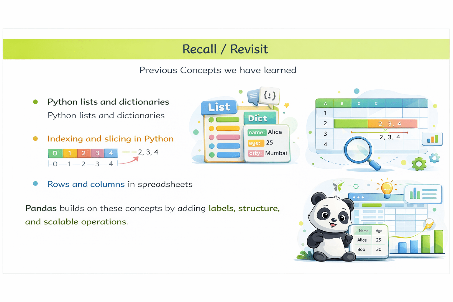
Pandas builds on these concepts by adding labels, structure, and scalable operations.
Every day, COVID data is released.
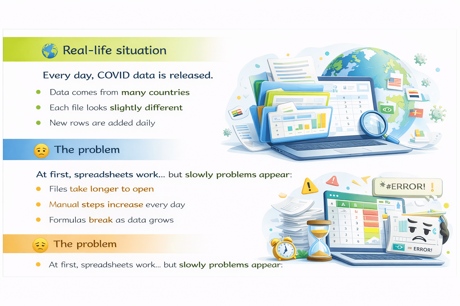
Data comes from many countries
Each file looks slightly different
New rows are added daily

The Problem

Real Life Situation

Files take longer to open
Manual steps increase every day
Formulas break when data grows
Now the data is...
Too large to manage by hand
Changing every day, so copy-paste fails
Too important to make mistakes
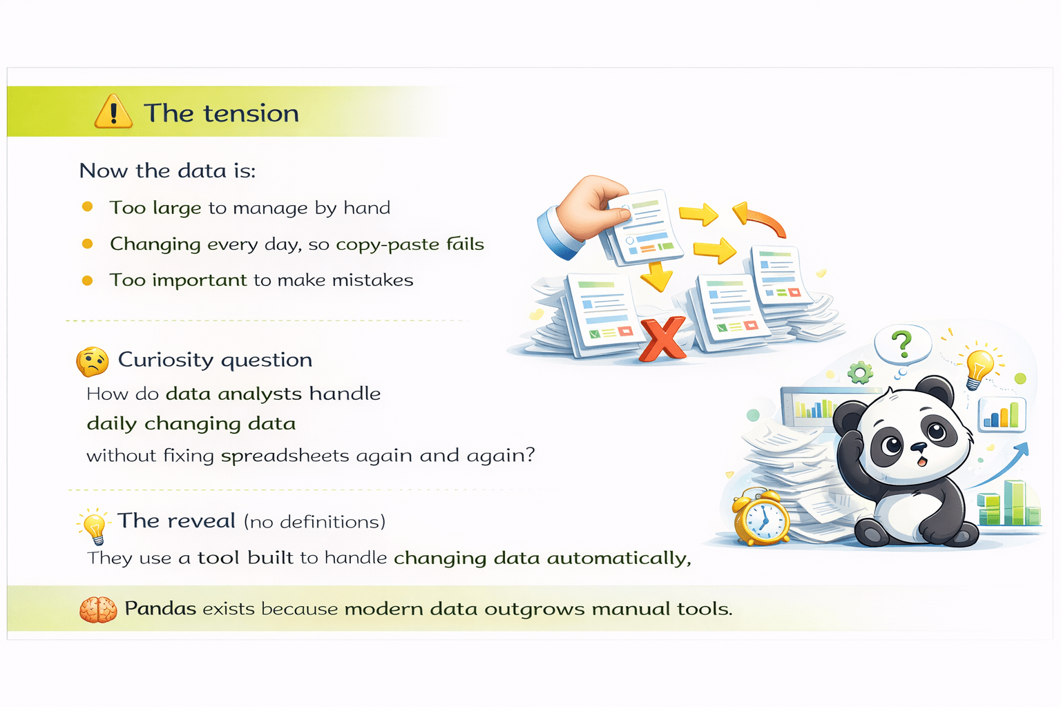
So how to Data Analysts handle daily changing data without fixing spreadsheets again and agian?
"Simply by using a tool designed to manipulate data."


Pandas exists because modern data outgrows manual tools.
Working with large and evolving datasets requires tools that can...
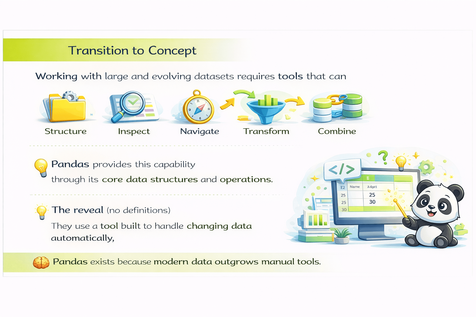
...data programmatically.
Pandas provides this capability through its core data structures and operations.

What is Pandas?
Explanation:
- Pandas is a Python library designed for efficient data manipulation and analysis.
- It provides high-level data structures that simplify working with structured data such as tables.

Key points

Used in data science, machine learning, and analytics
Optimized for large datasets
Works with tabular data formats


Primary data structures:
DataFrames
Series
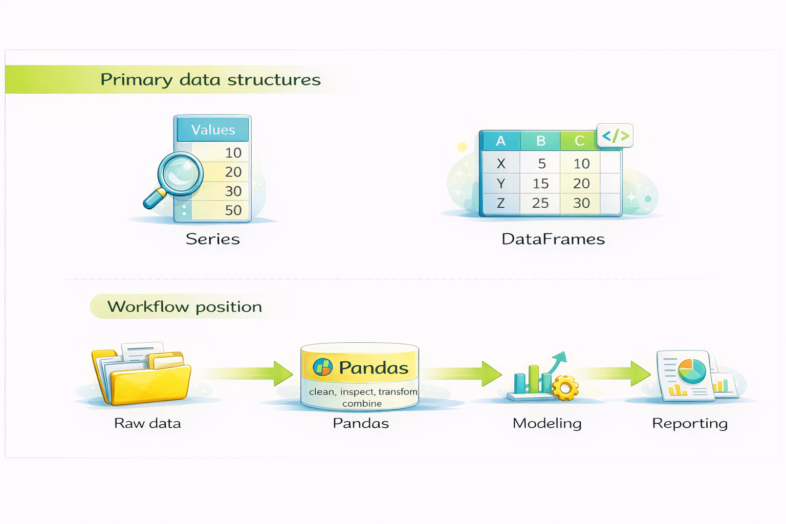
Workflow position:
Raw data
Pandas
Visualization/ Modeling
Report
Installing and Setting Up Pandas
Why installation matters
Before working with Series and DataFrames, Pandas must be installed correctly so that Python can access its data structures and functions.
Pandas is not part of Python’s standard library and must be installed separately.
Installing Pandas

-
Using pip
pip install pandas
Verifying Installation

import pandas as pd
print(pd.__version__)

output:
  3.0.0
latest version of pandas
Explanation:
Import pandas as pd loads the Pandas library
pd is the conventional alias used across the data ecosystem
Printing the version confirms successful installation
alias
Best practices

Always import Pandas at the top of the script or notebook
Use the standard alias pd for readability and consistency
Verify installation before starting data analysis
Pandas Series Overview
Explanation:
A Series represents a one-dimensional labeled array. It is comparable to a single column in a spreadsheet, where each value has an associated label called an index.

Key characteristics

One-dimensional
Index-based lables
Supports multiple data types (numbers, strings, dates, booleans)
Why series exists

Represents a single variable clearly
Enables label-based access instead of relying only on position
Foundation for DataFrames
- Multiple Series combine to form a DataFrame
Creating a Series

marks = pd.Series(
    [85, 90, 78, 92, 88],
    index=["Amit", "Priya", "Rahul", "Neha", "Ravi"]
)
Explanation of code:
- The list defines the data values
- The index assigns labels to each value
- Pandas stores both together as a Series
marks = pd.Series(
    [85, 90, 78, 92, 88],
    index=["Amit", "Priya", "Rahul", "Neha", "Ravi"]
)
marks = pd.Series(
    [85, 90, 78, 92, 88],
    index=["Amit", "Priya", "Rahul", "Neha", "Ravi"]
)
Accessing Series data
marks["Priya"]

output:
  75
Explanation
The value associated with the label "Priya" is returned directly.
Good Practices
- Use meaningful index labels
- Store only one variable per Series
Common issues
- Treating Series like plain Python lists
- Ignoring index alignment during operations
Pandas DataFrame Overview
Explanation
A DataFrame is a two-dimensional data structure composed of multiple Series aligned by a common index. It represents data in rows and columns.
Key characteristics
- Two-dimensional (rows and columns)
- Labeled rows and columns
- Columns can contain different data types
- Comparable to spreadsheets or SQL table

Why DataFrames exist
- Real-world datasets contain multiple related variables

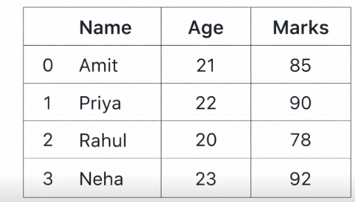
Creating a DataFrame
df = pd.DataFrame({
    "Name": ["Amit", "Priya", "Rahul", "Neha"],
    "Age": [21, 22, 20, 23],
    "Marks": [85, 90, 78, 92]
})
output:
    Name  Age  Marks
0   Amit   21     85
1  Priya   22     90
2  Rahul   20     78
3 Neha 23 92- Dictionary keys become column names
- Dictionary values become column data
- All columns are aligned into a single table
Explanation of code
Exploring DataFrames: head() and tail()
Purpose:
- Large datasets cannot be viewed entirely. These methods provide a quick overview.
Code:
df.head()
df.tail()
df.head(10)
df.tail(3)
Explanation:
- head() shows the first rows (default: 5)

- tail() shows the last rows (default: 5)
- Passing a number controls how many rows are displayed
Inspecting DataFrame Structure
Purpose:
- Understanding structure prevents incorrect assumptions during analysis.
Code:
Explanation:
import pandas as pd
d1 = pd.DataFrame({
    "name" : ['Sahil','Disha','Prem','Chandan'],
    "age" : [20,21,22,21]
})
print(d1.info())- Displays column names, data types, non-null counts, and memory usage.
Code:
import pandas as pd
d1 = pd.DataFrame({
    "name" : ['Sahil','Disha','Prem','Chandan'],
    "age" : [20,21,22,21]
})
print(d1.describe())

output:
               age
	count   4.000000
	mean   21.000000
	std     0.816497
	min    20.000000
	25%    20.750000
	50%    21.000000
	75%    21.250000
max 22.000000- Provides summary statistics such as count, mean, minimum, and maximum for numerical columns.
Explanation:
Inspecting DataFrame Structure
Single column
df["Marks"]
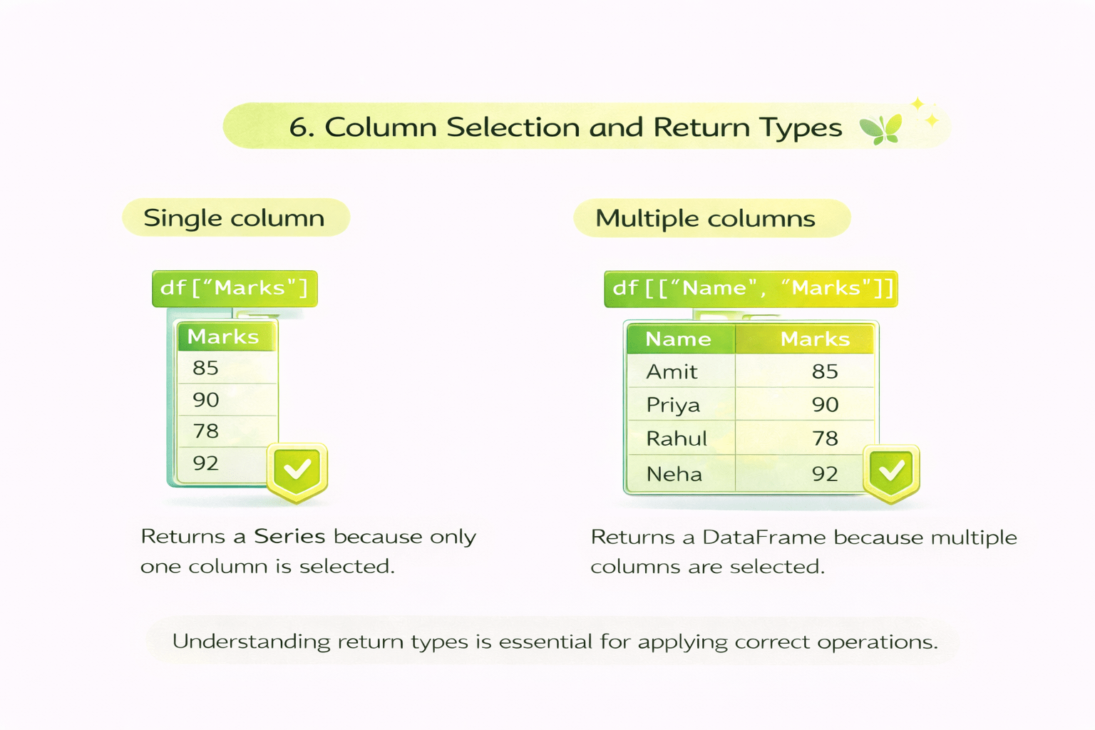
Explanation
Returns a Series because only one column is selected.
Multiple columns
df[["Name", "Marks"]]
Explanation
Returns a DataFrame because multiple columns are selected.
Understanding return types is essential for applying correct operations.

Label-Based Indexing using loc
Explanation:
- loc is used to access data using row and column labels.
Code:
df.loc[0, "Marks"]

output:
  np.int64(85)
Explanation:-
Returns the value from the row with label 0 and column "Marks".
Code:
df.loc[:, ['Name',"Marks"]]

output:
  	Name	Marks
0	Amit	85
1	Priya	90
2	Rahul	78
3	Neha	92
Explanation
Selects all rows and only the specified columns.
Best practice
- Use loc when labels are meaningful and readability is important.

Position-Based Indexing using iloc
Explanation:
- iloc accesses data using integer positions, starting from 0.
Code:
df.iloc[0, 2]

output:
  np.int64(85)
Explanation
- Returns the value at the first row and third column.
0 1 2
Code:
df.iloc[:, 1:3]

output:
  	Age	Marks
0	21	85
1	22	90
2	20	78
3	23	92
Explanation
- Selects all rows and columns at positions 1 and 2.
0 1 2
3 is exclusive so it will stop at 2
Filtering Data
Explanation:
-
Filtering extracts rows that meet specific conditions.
Code:
df[df["Marks"] > 80]

output:

	Name	Age	Marks
0	Amit	21	85
1	Priya	22	90
3	Neha	23	92
Explanation
-
The condition creates a Boolean mask
- Rows with True values are retained
Code:
df[(df["Marks"] > 80) & (df["Age"] > 21)]

output:

	Name	Age	Marks
1	Priya	22	90
3	Neha	23	92
Explanation
-
Multiple conditions are combined using logical operators.
Sorting Data
Explanation:
-
Sorting rearranges rows based on column values.
Code:
df.sort_values(by="Marks", ascending=False)

output:
  	Name	Age	Marks
3	Neha	23	92
1	Priya	22	90
0	Amit	21	85
2	Rahul	20	78
Explanation
-
Rows are ordered by Marks
-
Highest values appear first
Sorting changes row order but does not modify the index.
Resetting the Index
Explanation:
-
After filtering or sorting, index labels may no longer be sequential. Resetting the index restores a clean numeric index.
Code:
df.reset_index(drop=True, inplace=True)
Explanation
-
drop=True removes the old index
- A new index starting from 0 is created
Explanation:
filtered_df = df[df["Marks"] > 80]
print(filtered_df)

output:
    Name  Age  Marks
0   Amit   21     85
1  Priya   22     90
3   Neha   23     92
filtered_df.reset_index(drop=True, inplace=True)
print(filtered_df)
output:
Name Age Marks
0 Amit 21 85
1 Priya 22 90
2 Neha 23 92Concatenating DataFrames and SeriesResetting the Index
Explanation:
-
Data often exists in multiple parts. Concatenation combines them into a single structure.
Vertical concatenation (row-wise)
Code: pd.concat([df1, df2])
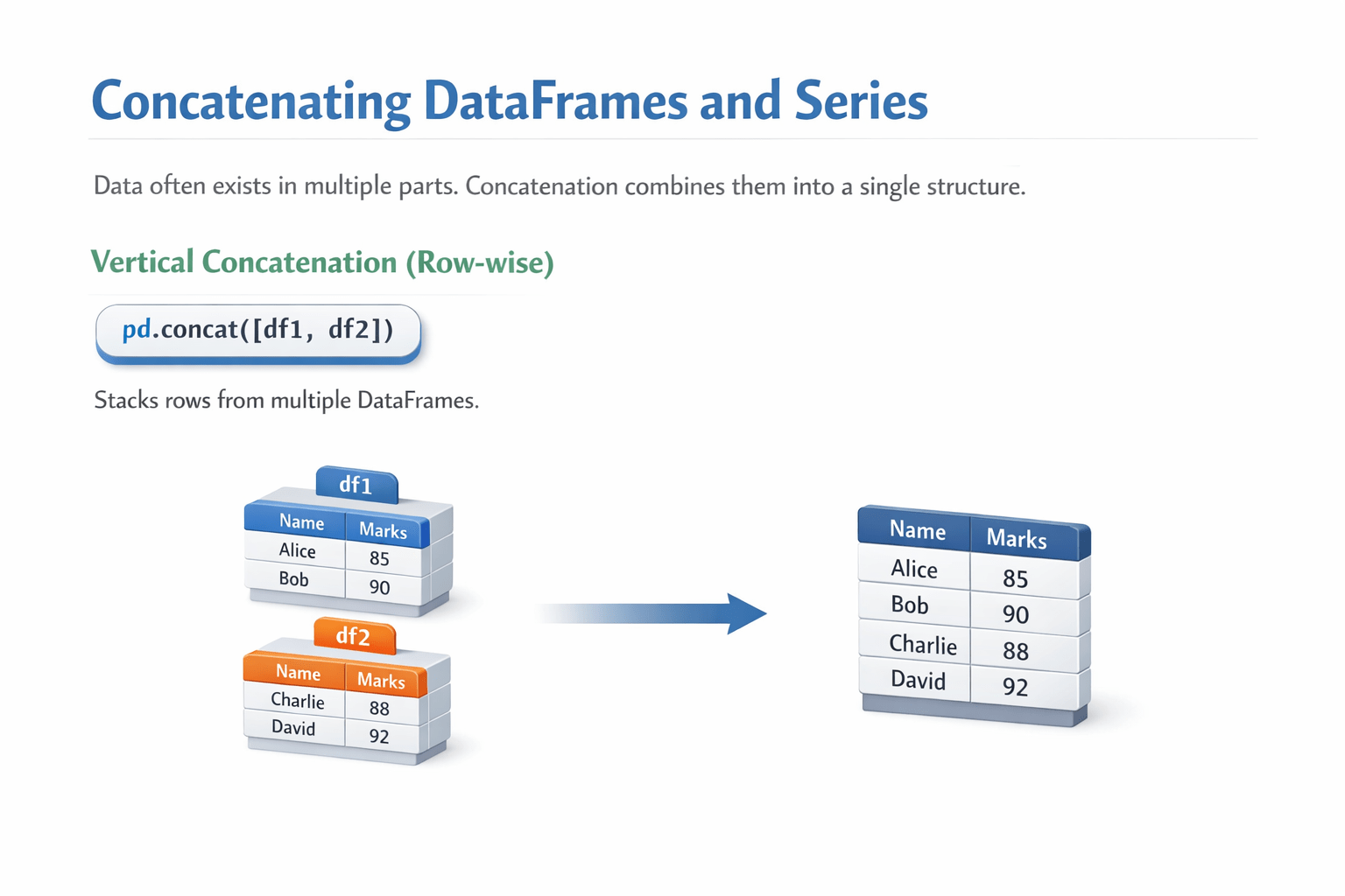
Explanation:
-
Stacks rows from multiple DataFrames.
Horizontal concatenation (column-wise)
Code: pd.concat([df1, df2], axis=1)
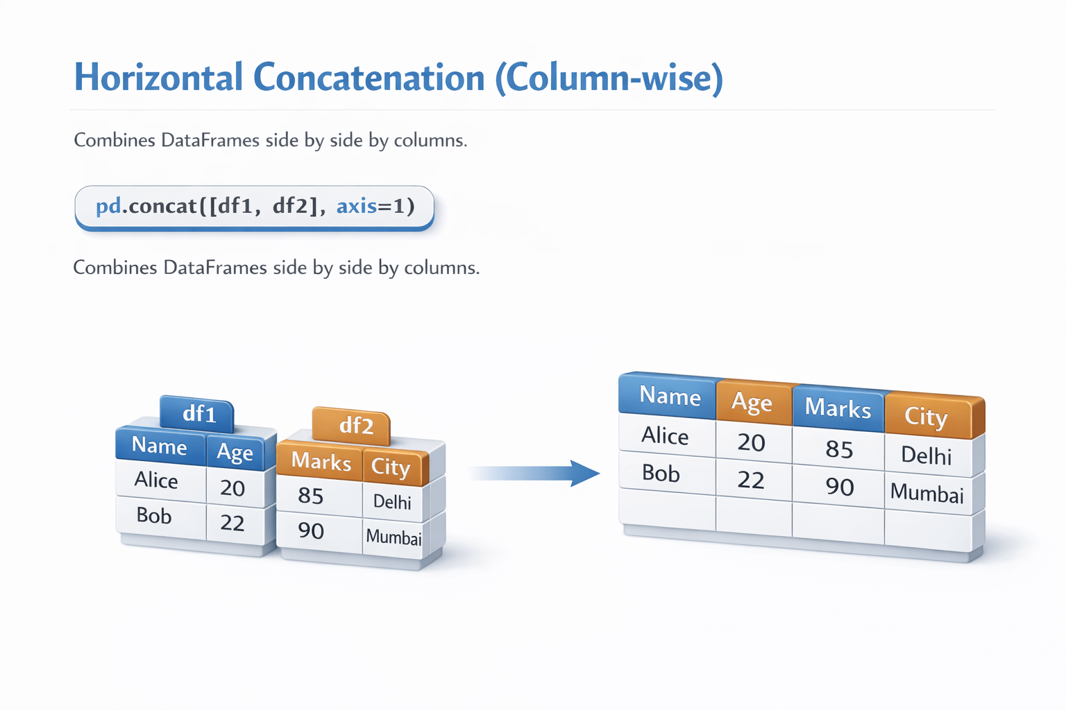
Explanation:
- Combines DataFrames side by side by columns.
Managing index
Code: pd.concat([df1, df2], ignore_index=True)
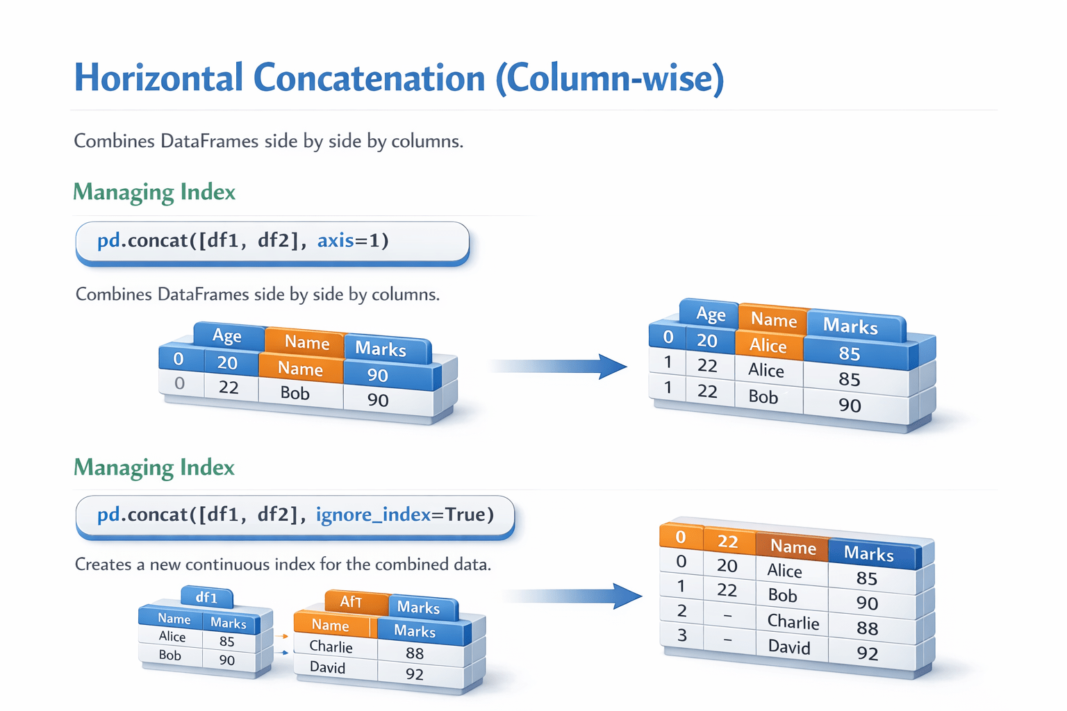
Explanation
- Creates a new continuous index for the combined data.
Relationship Between Series and DataFrames
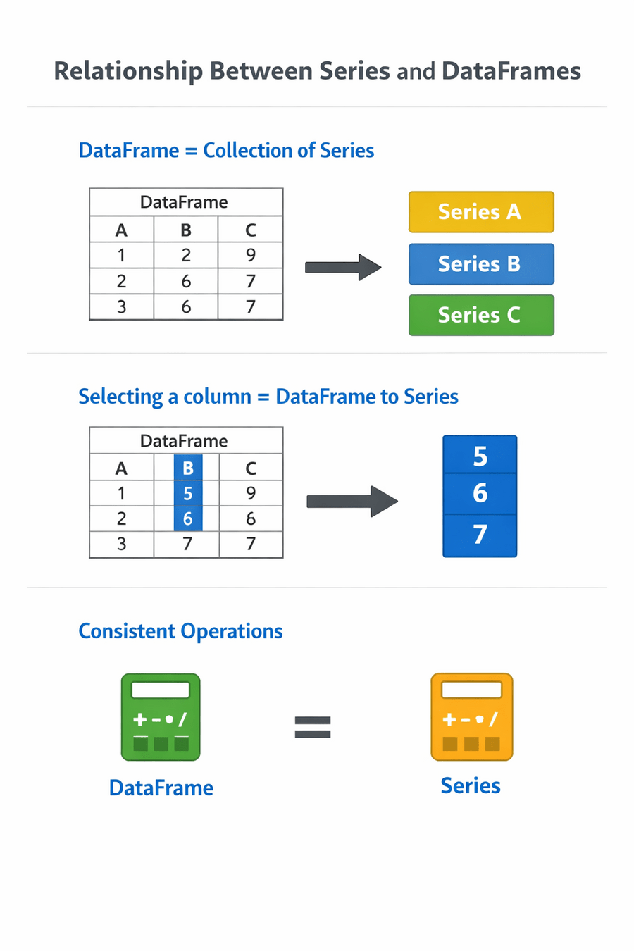
DataFrames are collections of Series
Selecting a column converts a DataFrame into a Series
Many operations work consistently across both structures
Summary
5
These concepts support reliable and scalable data workflows
4
Index management, and concatenation are essential operations
3
Inspection, navigation, filtering, sorting,
2
Series and DataFrames are foundational data structures
1
Pandas is a core Python library for data manipulation
Quiz
What is the primary purpose of pd.concat()?
A. Sorting data
B. Filtering data
C. Combining datasets
D. Resetting indexes

Quiz-Answer
C. Combining datasets

What is the primary purpose of pd.concat()?
A. Sorting data
B. Filtering data
D. Resetting indexes