Equation différentielle linéaire d'ordre 1

\left\{\begin{aligned} a: I & \rightarrow \mathbb{R} \\ x & \mapsto x \end{aligned}\right.

\(a\) est continue

I=\mathbb{R}

\left\{\begin{aligned} A: I & \rightarrow \mathbb{R} \\ x & \mapsto \dfrac{x^2}{2} \end{aligned}\right.

\(A\) est une primitive de \(a\)

\left\{\begin{aligned} b: I & \rightarrow \mathbb{R} \\ x & \mapsto x \end{aligned}\right.

\(b\) est continue

\mathcal{S}=\left\{\begin{aligned} y: I & \rightarrow \mathbb{R} \\ x & \mapsto \lambda e^{-A(x)} +y_p \end{aligned} ,\lambda \in\mathbb{R} \right\}

\(y_p\) est une solution particulière

Méthode de la variation de la constante:
On cherche \(y_p\) sous la forme \(y_p :x\mapsto \lambda(x) e^{-A(x)}\) avec \( \lambda\) dérivable sur \( I\)

\forall x\in I, \lambda'(x) =b(x)e^{A(x)}=xe^{\frac{x^2}{2}}

\text{ Donc, on choisit } \lambda(x) =e^{\frac{x^2}{2}} \\\text{ Et } y_p(x) = \lambda(x) e^{-A(x)}=e^{\frac{x^2}{2}}e^{-\frac{x^2}{2}}=1

\mathcal{S}=\left\{\begin{aligned} y: I & \rightarrow \mathbb{R} \\ x & \mapsto \lambda e^{-\frac{x^2}{2}} +1 \end{aligned} ,\lambda \in\mathbb{R} \right\}

\left\{\begin{aligned} a: I & \rightarrow \mathbb{R} \\ x & \mapsto x \end{aligned}\right.

\(a\) est continue

I=\mathbb{R}

\left\{\begin{aligned} A: I & \rightarrow \mathbb{R} \\ x & \mapsto \dfrac{x^2}{2} \end{aligned}\right.

\(A\) est une primitive de \(a\)

\left\{\begin{aligned} b: I & \rightarrow \mathbb{R} \\ x & \mapsto x +\cos(x)e^{-\frac{x^2}{2}}\end{aligned}\right.

\(b\) est continue

\mathcal{S}=\left\{\begin{aligned} y: I & \rightarrow \mathbb{R} \\ x & \mapsto \lambda e^{-A(x)} +y_p \end{aligned} ,\lambda \in\mathbb{R} \right\}

\(y_p\) est une solution particulière

Méthode de la variation de la constante:
On cherche \(y_p\) sous la forme \(y_p :x\mapsto \lambda(x) e^{-A(x)}\) avec \( \lambda\) dérivable sur \( I\)

\forall x\in I, \lambda'(x) =b(x)e^{A(x)}=(x +\cos(x)e^{-\frac{x^2}{2}})e^{\frac{x^2}{2}}= xe^{\frac{x^2}{2}}+ \cos(x)

\mathcal{S}=\left\{\begin{aligned} y: I & \rightarrow \mathbb{R} \\ x & \mapsto \lambda e^{-\frac{x^2}{2}} +1+\sin(x)e^{-\frac{x^2}{2}} \end{aligned} ,\lambda \in\mathbb{R} \right\}

\text{ Donc, on choisit } \lambda(x) =e^{\frac{x^2}{2}} +\sin(x)\\\text{ Et } y_p(x) = \lambda(x) e^{-A(x)}=\left(e^{\frac{x^2}{2}}+\sin(x)\right)e^{-\frac{x^2}{2}}=1+\sin(x)e^{-\frac{x^2}{2}}

\mathcal{S}=\left\{\begin{aligned} y: \mathbb{R} & \rightarrow \mathbb{R} \\ x & \mapsto \lambda e^{-\frac{x}{RC}} +E \end{aligned} ,\lambda \in\mathbb{R} \right\}

Exercice 4

\dfrac{e^x}{(e^x-1)^2} -\dfrac{e^x}{e^x-1} +1 \\= \dfrac{e^x}{(e^x-1)^2} -\dfrac{e^x(e^x-1)}{(e^x-1)^2} +\dfrac{(e^x-1)^2}{(e^x-1)^2} \\= \dfrac{e^x-e^x(e^x-1)+(e^x-1)^2}{(e^x-1)^2} \\= \dfrac{e^x-e^{2x}+e^x+e^{2x}-2e^x+1}{(e^x-1)^2} \\= \dfrac{1}{(e^x-1)^2}

Exercice 4

(E)\iff y'=\dfrac{e^x}{(e^x-1)^2} -\dfrac{e^x}{e^x-1} +1

\text{Donc, sur } \mathbb{R}_+^* , y(x)= -\dfrac{1}{e^x-1} -\ln( e^x-1 )+x+\lambda

\text{Et, sur } \mathbb{R}_-^* , y(x)= -\dfrac{1}{e^x-1} -\ln( 1- e^x )+x+\lambda

\mathcal{S_+}=\left\{\begin{aligned} y: \mathbb{R}_+^* & \rightarrow \mathbb{R} \\ x & \mapsto -\dfrac{1}{e^x-1} -\ln( e^x-1 )+x+\lambda \end{aligned} ,\lambda \in\mathbb{R} \right\}

\mathcal{S_-}=\left\{\begin{aligned} y: \mathbb{R}_-^* & \rightarrow \mathbb{R} \\ x & \mapsto -\dfrac{1}{e^x-1} -\ln( 1-e^x )+x+\lambda \end{aligned} ,\lambda \in\mathbb{R} \right\}

\left\{\begin{aligned} a: I & \rightarrow \mathbb{R} \\ x & \mapsto \dfrac{e^x}{1-e^x} \end{aligned}\right.

\(a\) est continue

\text{cas 1: }I=\mathbb{R}_+^*

\left\{\begin{aligned} A: I & \rightarrow \mathbb{R} \\ x & \mapsto -\ln\left( \vert 1-e^x\vert\right)= -\ln\left( e^x-1\right)\end{aligned}\right.

\(A\) est une primitive de \(a\)

\left\{\begin{aligned} b: I & \rightarrow \mathbb{R} \\ x & \mapsto \dfrac{1}{e^x-1}\end{aligned}\right.

\(b\) est continue

\mathcal{S}=\left\{\begin{aligned} y: I & \rightarrow \mathbb{R} \\ x & \mapsto \lambda e^{-A(x)} +y_p \end{aligned} ,\lambda \in\mathbb{R} \right\}

\(y_p\) est une solution particulière

Méthode de la variation de la constante:
On cherche \(y_p\) sous la forme \(y_p :x\mapsto \lambda(x) e^{-A(x)}\) avec \( \lambda\) dérivable sur \( I\)

\forall x\in I, \lambda'(x) =b(x)e^{A(x)}= \dfrac{1}{e^x-1} e^{-\ln(e^x-1)} = \dfrac{1}{(e^x-1)^2} =\dfrac{e^x}{(e^x-1)^2} -\dfrac{e^x}{e^x-1} +1

\mathcal{S_+}=\left\{\begin{aligned} y: \mathbb{R}_+^* & \rightarrow \mathbb{R} \\ x & \mapsto (e^x-1)\left( \lambda +x-\ln(e^x-1)-\dfrac{1}{e^x-1} \right) \end{aligned} ,\lambda \in\mathbb{R} \right\}

\text{ Donc , on choisit } \lambda(x) =-\dfrac{1}{e^x-1}-\ln(e^x-1)+x

Exercice 4

\left\{\begin{aligned} a: I & \rightarrow \mathbb{R} \\ x & \mapsto \dfrac{e^x}{1-e^x} \end{aligned}\right.

\(a\) est continue

\text{cas 2: }I=\mathbb{R}_-^*

\left\{\begin{aligned} A: I & \rightarrow \mathbb{R} \\ x & \mapsto -\ln\left( \vert 1-e^x\vert\right)= -\ln\left( 1-e^x\right)\end{aligned}\right.

\(A\) est une primitive de \(a\)

\left\{\begin{aligned} b: I & \rightarrow \mathbb{R} \\ x & \mapsto \dfrac{1}{e^x-1}\end{aligned}\right.

\(b\) est continue

\mathcal{S}=\left\{\begin{aligned} y: I & \rightarrow \mathbb{R} \\ x & \mapsto \lambda e^{-A(x)} +y_p \end{aligned} ,\lambda \in\mathbb{R} \right\}

\(y_p\) est une solution particulière

Méthode de la variation de la constante:
On cherche \(y_p\) sous la forme \(y_p :x\mapsto \lambda(x) e^{-A(x)}\) avec \( \lambda\) dérivable sur \( I\)

\forall x\in I, \lambda'(x) =b(x)e^{A(x)}= \dfrac{1}{e^x-1} e^{-\ln(1-e^x)} =- \dfrac{1}{(e^x-1)^2} =-\dfrac{e^x}{(e^x-1)^2} +\dfrac{e^x}{e^x-1} -1

\mathcal{S_-}=\left\{\begin{aligned} y: \mathbb{R}_-^* & \rightarrow \mathbb{R} \\ x & \mapsto (1-e^x)\left( \lambda -x+\ln(1-e^x)+\dfrac{1}{e^x-1} \right) \end{aligned} ,\lambda \in\mathbb{R} \right\}

\text{ Donc , on choisit } \lambda(x) =\dfrac{1}{e^x-1}+\ln(1-e^x)-x

Exercice 4

(E) \iff y' +\dfrac{x}{x-1} y=x+1

\left\{\begin{aligned} a: I & \rightarrow \mathbb{R} \\ x & \mapsto \dfrac{e^x}{1-e^x} \end{aligned}\right.

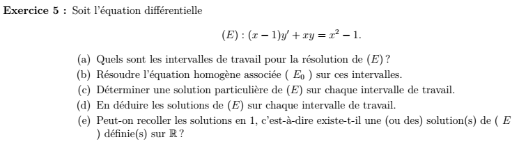
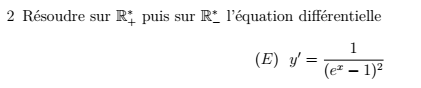
\(a\) est continue sur \(\mathbb{R}\setminus\{1\}\)

donc \(I=]-\infty,1[\) ou \(I=]1,+\infty[\)

(E_0) \iff y' +\dfrac{x}{x-1} y=0

\left\{\begin{aligned} a: I & \rightarrow \mathbb{R} \\ x & \mapsto 1+\dfrac{1}{x-1} \end{aligned}\right.

\(a\) est continue sur \(\ I\)

pour \(I=]1,+\infty[\)

pour \(I=]-\infty,1[\)

\left\{\begin{aligned} A: I & \rightarrow \mathbb{R} \\ x & \mapsto x+ \ln(1-x) \end{aligned}\right.

\left\{\begin{aligned} A: I & \rightarrow \mathbb{R} \\ x & \mapsto x+ \ln(x-1) \end{aligned}\right.

\mathcal{S_0}=\left\{\begin{aligned} y: I & \rightarrow \mathbb{R} \\ x & \mapsto \dfrac{\lambda e^{-x}}{1-x} \end{aligned} ,\lambda \in\mathbb{R} \right\}

\mathcal{S_0}=\left\{\begin{aligned} y: I & \rightarrow \mathbb{R} \\ x & \mapsto \dfrac{\lambda e^{-x}}{x-1} \end{aligned} ,\lambda \in\mathbb{R} \right\}

(E) \iff y' +\dfrac{x}{x-1} y=x+1

pour \(I=]1,+\infty[\)

pour \(I=]-\infty,1[\)

\left\{\begin{aligned} A: I & \rightarrow \mathbb{R} \\ x & \mapsto x+ \ln(1-x) \end{aligned}\right.

\left\{\begin{aligned} A: I & \rightarrow \mathbb{R} \\ x & \mapsto x+ \ln(x-1) \end{aligned}\right.

Méthode de la variation de la constante:
On cherche \(y_p\) sous la forme \(y_p :x\mapsto \lambda(x) e^{-A(x)}\) avec \( \lambda\) dérivable sur \( I\)

\forall x\in I, \lambda'(x) =b(x)e^{A(x)}=(1-x^2) e^x

\text{ Donc , on choisit } \lambda(x) =-(x-1)^2 e^x

\forall x\in I, \lambda'(x) =b(x)e^{A(x)}=(x^2-1) e^x

\text{ Donc , on choisit } \lambda(x) =(x-1)^2 e^x

y_p :x\mapsto -(x-1)^2e^x e^{-x-\ln(1-x)}

y_p :x\mapsto x-1

y_p :x\mapsto (x-1)^2e^x e^{-x-\ln(x-1)}

y_p :x\mapsto x-1

pour \(I=]1,+\infty[\)

pour \(I=]-\infty,1[\)

\mathcal{S}=\left\{\begin{aligned} y: I & \rightarrow \mathbb{R} \\ x & \mapsto \dfrac{\lambda e^{-x}}{1-x} +x-1 \end{aligned} ,\lambda \in\mathbb{R} \right\}

\mathcal{S}=\left\{\begin{aligned} y: I & \rightarrow \mathbb{R} \\ x & \mapsto \dfrac{\lambda e^{-x}}{x-1} +x-1 \end{aligned} ,\lambda \in\mathbb{R} \right\}

\mu=-\lambda

\mathcal{S}=\left\{\begin{aligned} y: I & \rightarrow \mathbb{R} \\ x & \mapsto \dfrac{\mu e^{-x}}{x-1} +x-1 \end{aligned} ,\mu \in\mathbb{R} \right\}

Soit

f_{\mu,\lambda} : x\mapsto \left\{\begin{aligned} \dfrac{\mu e^{-x}}{x-1} +x-1& \text{ ~~si }x<1\\\\ \dfrac{\lambda e^{-x}}{x-1} +x-1& \text{ ~~si }x<1 \end{aligned} \right.

Existe -il un couple \( (\lambda,\mu) \) tel que \( \tilde{f}_{\lambda,\mu} \) soit de classe \(\mathcal{C_1}(\mathbb{R})\) ?

f_{\mu,\lambda} : x\mapsto \left\{\begin{aligned} \dfrac{\mu e^{-x}}{x-1} +x-1& \text{ ~~si }x<1\\\\ \dfrac{\lambda e^{-x}}{x-1} +x-1& \text{ ~~si }x>1 \end{aligned} \right.

\(f_{\lambda,\mu} \) est de classe \(\mathcal{C_1}(\mathbb{]-\infty;1[}) \)
\(f_{\lambda,\mu} \) est de classe \(\mathcal{C_1}(\mathbb{]1;\infty[})\)
\(\lim\limits_{x\to 1^-} \frac{e^{-x}}{x-1}=-\infty\)
\(\lim\limits_{x\to 1^+} \frac{e^{-x}}{x-1}=+\infty\)

\( \tilde{f}_{0,0} \) est classe \(\mathcal{C_1}(\mathbb{R})\)

f_{0,0} : x\mapsto \left\{\begin{aligned} x-1& \text{ ~~si }x<1\\\\ x-1& \text{ ~~si }x>1 \end{aligned} \right.

\text{Le seul couple \( (\lambda,\mu) \) permettant un prolongement par continuité en 1 est le couple (0,0) .}\\ \tilde{f}_{0,0} : x\mapsto x-1

\left\{\begin{aligned} a: I & \rightarrow \mathbb{R} \\ x & \mapsto \dfrac{\sin(x)}{\cos(x)} \end{aligned}\right.

\(a\) est continue

\left\{\begin{aligned} A: I & \rightarrow \mathbb{R} \\ x & \mapsto -\ln\left( \vert \cos(x) \vert\right)= -\ln\left( \cos(x)\right)\end{aligned}\right.

\(A\) est une primitive de \(a\)

\left\{\begin{aligned} b: I & \rightarrow \mathbb{R} \\ x & \mapsto \sin(2x) \end{aligned}\right.

\(b\) est continue

\mathcal{S}=\left\{\begin{aligned} y: I & \rightarrow \mathbb{R} \\ x & \mapsto \lambda e^{-A(x)} +y_p \end{aligned} ,\lambda \in\mathbb{R} \right\}

\(y_p\) est une solution particulière

Méthode de la variation de la constante:
On cherche \(y_p\) sous la forme \(y_p :x\mapsto \lambda(x) e^{-A(x)}\) avec \( \lambda\) dérivable sur \( I\)

\forall x\in I, \lambda'(x) =b(x)e^{A(x)}= \sin(2x) e^{-\ln(\cos(x))} = 2\sin(x)

\mathcal{S}=\left\{\begin{aligned} y: ]-\dfrac{\pi}{2},\dfrac{\pi}{2}[ & \rightarrow \mathbb{R} \\ x & \mapsto \cos(x) \left( \lambda -2\cos(x) \right) \end{aligned} ,\lambda \in\mathbb{R} \right\}

\text{ Donc , on choisit } \lambda(x) = -2\cos(x)

I=]-\dfrac{\pi}{2},\dfrac{\pi}{2}[

\left\{\begin{aligned} a: I & \rightarrow \mathbb{R} \\ x & \mapsto -\dfrac{1}{x(x^2+1)}= -\dfrac{1}{x}+\dfrac{x}{x^2+1} \end{aligned}\right.

\(a\) est continue

\left\{\begin{aligned} A: I & \rightarrow \mathbb{R} \\ x & \mapsto -\ln\left( \vert x \vert\right)+\dfrac{1}{2} \ln\left( 1+x^2\right)\end{aligned}\right.

\(A\) est une primitive de \(a\)

\left\{\begin{aligned} b: I & \rightarrow \mathbb{R} \\ x & \mapsto \dfrac{\sqrt{1+x^2}}{x} \end{aligned}\right.

\(b\) est continue

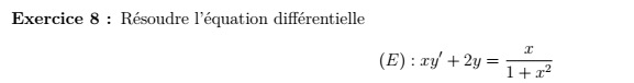
Les intervalles I de travail sont \(]-\infty,0[\) et \(]0,+\infty[\)

Méthode de la variation de la constante:
On cherche \(y_p\) sous la forme \(y_p :x\mapsto \lambda(x) e^{-A(x)}\) avec \( \lambda\) dérivable sur \( I\)

\forall x\in I, \lambda'(x) =b(x)e^{A(x)}= -\dfrac{1+x^2}{x^2} = -\dfrac{1}{x^2}-1

\mathcal{S_-}=\left\{\begin{aligned} y: I & \rightarrow \mathbb{R} \\ x & \mapsto \left( \mu - \dfrac{1}{x}+x\right)\dfrac{x}{\sqrt{1+x^2}} \end{aligned} ,\mu \in\mathbb{R} \right\}

\text{ Donc , on choisit } \lambda(x) = \dfrac{1}{x}-x

Pour \(I=]-\infty,0[\)

\left\{\begin{aligned} A: I & \rightarrow \mathbb{R} \\ x & \mapsto -\ln\left( -x\right)+\dfrac{1}{2} \ln\left( 1+x^2\right) = \ln\left(-\dfrac{\sqrt{1+x^2}}{x}\right) \end{aligned}\right.

Méthode de la variation de la constante:
On cherche \(y_p\) sous la forme \(y_p :x\mapsto \lambda(x) e^{-A(x)}\) avec \( \lambda\) dérivable sur \( I\)

\forall x\in I, \lambda'(x) =b(x)e^{A(x)}= \dfrac{1+x^2}{x^2} = \dfrac{1}{x^2}+1

\mathcal{S_+}=\left\{\begin{aligned} y: I & \rightarrow \mathbb{R} \\ x & \mapsto \left( \lambda - \dfrac{1}{x}+x\right)\dfrac{x}{\sqrt{1+x^2}} \end{aligned} ,\lambda \in\mathbb{R} \right\}

\text{ Donc , on choisit } \lambda(x) = -\dfrac{1}{x}+x

Pour \(I=]0;+\infty[\)

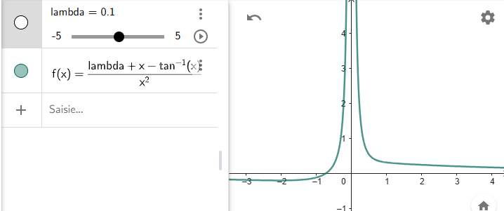
\left\{\begin{aligned} A: I & \rightarrow \mathbb{R} \\ x & \mapsto -\ln\left( x\right)+\dfrac{1}{2} \ln\left( 1+x^2\right) = \ln\left(\dfrac{\sqrt{1+x^2}}{x}\right) \end{aligned}\right.

Soit

\mathcal{S_-}=\left\{\begin{aligned} y: ]-\infty;0[ & \rightarrow \mathbb{R} \\ x & \mapsto \left( \mu - \dfrac{1}{x}+x\right)\dfrac{x}{\sqrt{1+x^2}} \end{aligned} ,\mu \in\mathbb{R} \right\}

\mathcal{S_+}=\left\{\begin{aligned} y: ]0;+\infty[ & \rightarrow \mathbb{R} \\ x & \mapsto \left( \lambda - \dfrac{1}{x}+x\right)\dfrac{x}{\sqrt{1+x^2}} \end{aligned} ,\lambda \in\mathbb{R} \right\}

On a trouvé :

f_{\mu,\lambda} : x\mapsto \left\{\begin{aligned} \left( \mu - \dfrac{1}{x}+x\right)\dfrac{x}{\sqrt{1+x^2}} & \text{ ~~si }x<0\\\\ \left( \lambda - \dfrac{1}{x}+x\right)\dfrac{x}{\sqrt{1+x^2}} & \text{ ~~si }x>0 \end{aligned} \right.

Etape 1:Existe -il un couple \( (\lambda,\mu) \) tel que \( f_{\lambda,\mu} \) soit prolongeable par continuité en 0 .

Etape 2:Déterminer les couples tels que \( \tilde{f}_{\lambda,\mu} \) soit de classe \(\mathcal{C_1}(\mathbb{R})\) ?

\text{Pour tout couple} (\lambda,\mu) , \lim\limits_{x\to 0^-}f_{\mu,\lambda} (x)= -1 \text{ ~~~ et ~~~} \lim\limits_{x\to 0^+}f_{\mu,\lambda} (x)= -1

Donc ,pour tout couple \((\lambda,\mu)\), il existe le prolongement par continuité suivant:

\tilde{f}_{\mu,\lambda} : x\mapsto \left\{\begin{aligned} \left( \mu x +x^2-1\right)\dfrac{1}{\sqrt{1+x^2}} & \text{ ~~si }x<0\\ -1 & \text{ ~~si }x=0\\ \left( \lambda x+x^2 -1\right)\dfrac{1}{\sqrt{1+x^2}} & \text{ ~~si }x>0 \end{aligned} \right.

f_{\mu,\lambda} : x\mapsto \left\{\begin{aligned} \left( \mu x +x^2-1\right)\dfrac{1}{\sqrt{1+x^2}} & \text{ ~~si }x<0\\ \left( \lambda x+x^2 -1\right)\dfrac{1}{\sqrt{1+x^2}} & \text{ ~~si }x>0 \end{aligned} \right.

Existe -il un couple \( (\lambda,\mu) \) tel que \( \tilde{f}_{\lambda,\mu} \) soit de classe \(\mathcal{C_1}(\mathbb{R})\) ?

Etant issue d'opérations sur des fonctions de classe \(\mathcal{C_1}\)
\( \tilde{f}_{\lambda,\mu}\) est de classe \(\mathcal{C_1}\)
sur \(\mathbb{R}_-^*\) et sur sur \(\mathbb{R}_+^*\)

On sait que \( \tilde{f}_{\lambda,\mu} \) est de classe \(\mathcal{C_0}(\mathbb{R})\)

Etude de la dérivabilité en 0 avec des \(DL_1(0^-)\) et \(DL_1(0^+)\) et :

\text{On sait que :~~}\dfrac{1}{\sqrt{1+x^2}}=(1+x^2)^{-\frac{1}{2}}\underset{0}{=}1-\frac{1}{2}x^2+o(x^2) \underset{0}{=} 1+o(x)

\text{Donc , }\tilde{f}_{\mu,\lambda} (x)\underset{0^-}{=}\left( \mu x +x^2-1\right) (1+o(x)) \underset{0^-}{=}-1+\mu x +o(x)

\tilde{f}_{\mu,\lambda} (x)\underset{0^+}{=}\left( \lambda x +x^2-1\right) (1+o(x)) \underset{0^+}{=}-1+\lambda x +o(x)

\( \tilde{f}_{\lambda,\mu} \) est dérivable en 0 si et seulement \( \lambda=\mu \)

\tilde{f}_{\lambda,\lambda}': x\mapsto \left\{\begin{aligned} \left(\lambda +2x\right)\dfrac{1}{\sqrt{1+x^2}} - \left(\lambda x+x^2-1\right)\dfrac{x}{(1+x^2)\sqrt{1+x^2}} & \text{ ~~si }x\neq 0\\ \lambda~~~~~~ & \text{ ~~si }x=0 \end{aligned} \right.

\text{Pour tout } \lambda , \lim\limits_{x\to 0}f_{\lambda,\lambda}' (x)= \lambda =f_{\lambda,\lambda}'(0)

\text{Donc } , f_{\lambda,\lambda}' \text{~~est continue sur } \mathbb{R}

\left\{\begin{aligned} a: I & \rightarrow \mathbb{R} \\ x & \mapsto \dfrac{2}{x} \end{aligned}\right.

\(a\) est continue

\left\{\begin{aligned} A: I & \rightarrow \mathbb{R} \\ x & \mapsto 2\ln\left( \vert x \vert\right)\end{aligned}\right.

\(A\) est une primitive de \(a\)

\left\{\begin{aligned} b: I & \rightarrow \mathbb{R} \\ x & \mapsto \dfrac{1}{1+x^2} \end{aligned}\right.

\(b\) est continue

\mathcal{S}=\left\{\begin{aligned} y: I & \rightarrow \mathbb{R} \\ x & \mapsto \dfrac{\lambda+x-\arctan(x)}{x^2} \end{aligned} ,\lambda \in\mathbb{R} \right\}

I=?\\ \cdots

\mathcal{S}=\left\{\begin{aligned} y: I & \rightarrow \mathbb{R} \\ x & \mapsto \dfrac{\lambda+x-\arctan(x)}{x^2} \end{aligned} ,\lambda \in\mathbb{R} \right\}

The end