{\color{red} {\text{Ordinary differential equations and partial differential equations
}}}
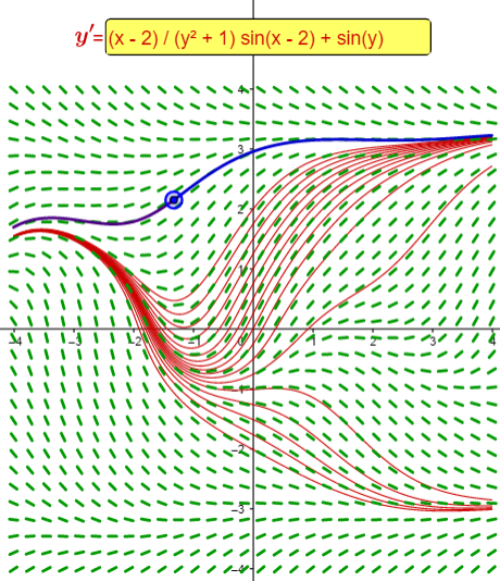
\text{Let us study this family of differential equations.}
\text{frequently, this equation will have the special form}
\text{(Note that in this method of separation of variables does not require } \\
\text{ the differential equation to be \textbf{linear})}
\displaystyle \frac{d y}{d x}=f(x, y)=-\frac{P(x, y)}{Q(x, y)} .
\displaystyle \frac{d y}{d x}=f(x, y)=-\frac{P(x)}{Q(y)} \text {. }
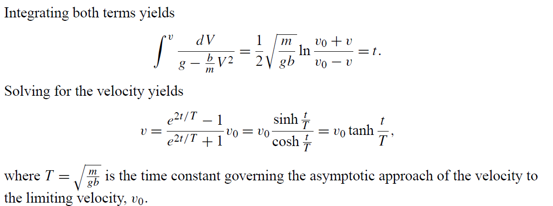
\text{Example: a falling object in presence of air drag}\\
\text{The equation of motion is: }
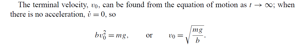
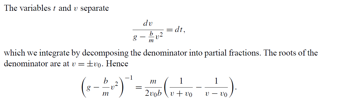
m \dot{v}=m g-b v^2
Exact differential equations
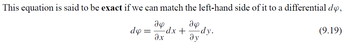
\text{in this case, we look at an unnknown function } \varphi(x,y)=\text{constant } d\varphi=0
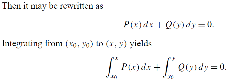
P(x, y) d x+Q(x, y) d y=0 .
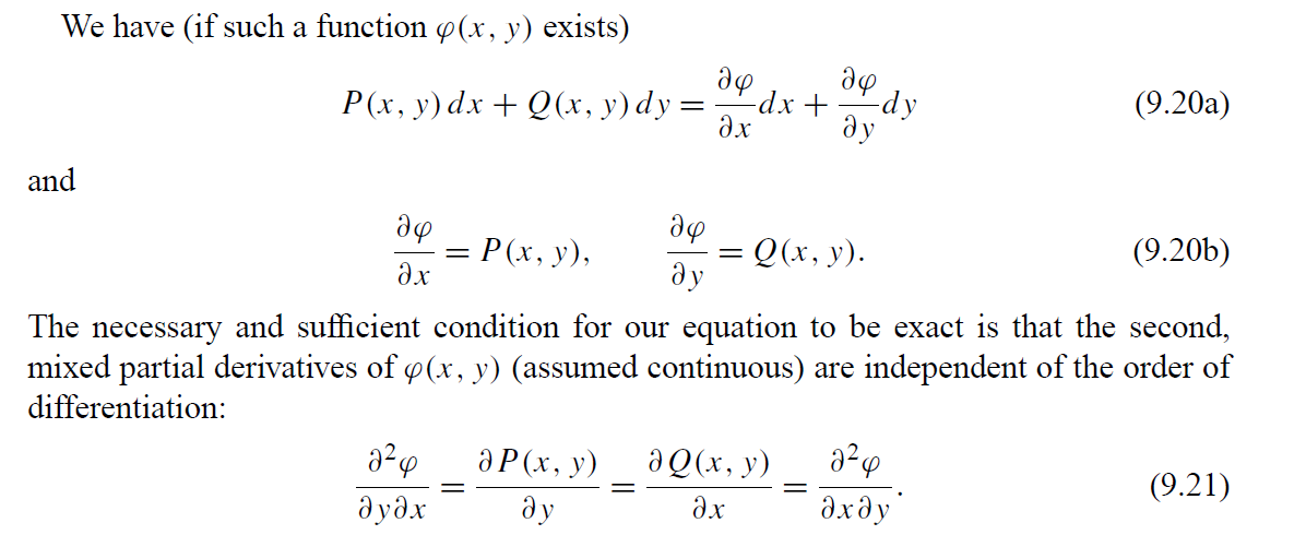
\displaystyle P(x,y) dx+Q(x,y) dy=0\\
\text{If the following differential equation is exact}\\
\text{the solution is}\\
\displaystyle \phi(x,y) =\int_{x_0}^x P(x,y) dx+\int_{y_0}^y Q({\color{red}{x_0}},y) dy=\text{constant}
\text{{\color{red}Equations of non-constant coefficients with missing y-term }}
{\color{red}y^{''}+p(x) y^{'}=f(x), \hspace{1cm} Q(x)=0}
\text{When Q(x)=0, the second order ODE can be converted into a first order linear equation.}
\text{The solution is therefore obtained following the simple steps below: }
\text{1) Substitute: } u=y^{'}, u^{'}=y^{''}, \hspace{1cm} u^{'}+p(x)u= f(x)\\
\text{2) Solve the ODE and get } u(x), \text{ following your preffered method (variation of conastant, ..)}
\text{3) Integrate to obtain y(x) }, \displaystyle{y(x)=\int^x u(x^{\prime}) dx^{\prime}}
\text{{\color{red}Example:}}
\text{Solve the following second order ODE: }\\xy^{''}+4y^{'}=x^2
\text{{\color{red} Solution:}}
\text{The standard form of the equation is: }
\displaystyle y^{''}+\frac{4}{x}y=x
\text{We substitute } u=y^{'} \text{ to get the new 1st order ODE: } \displaystyle u^{'}+\frac{4}{x}u=x
\text{The homogeneous solution is } \displaystyle u_h(x)=\frac{c}{x^4}
\text{To get the solution with the sourse term, we use the variation of constant method: } c\rightarrow c(x)
\displaystyle u^{'}(x)=c^{'}(x) \frac{1}{x^4}-4\frac{c(x)}{x^5}
\text{By injecting the obtained result in the equation we get: } \displaystyle c(x)=\Big(\frac{x^6}{6}+c_1\Big)
\displaystyle u(x)=\Big(\frac{x^6}{6}+c_1\Big)\frac{1}{x^4}
\text{The final solution is:}
\displaystyle y(x)=\int^x u(x^{'}) dx^{'}=\frac{x^3}{18}-\frac{c_1}{3x^3}+c_2
\text{{\color{red}{Remark: }}} \text{the method works regardless the ODE is homogeneous or not, or with constant}\\ \text{ parameters or not.}
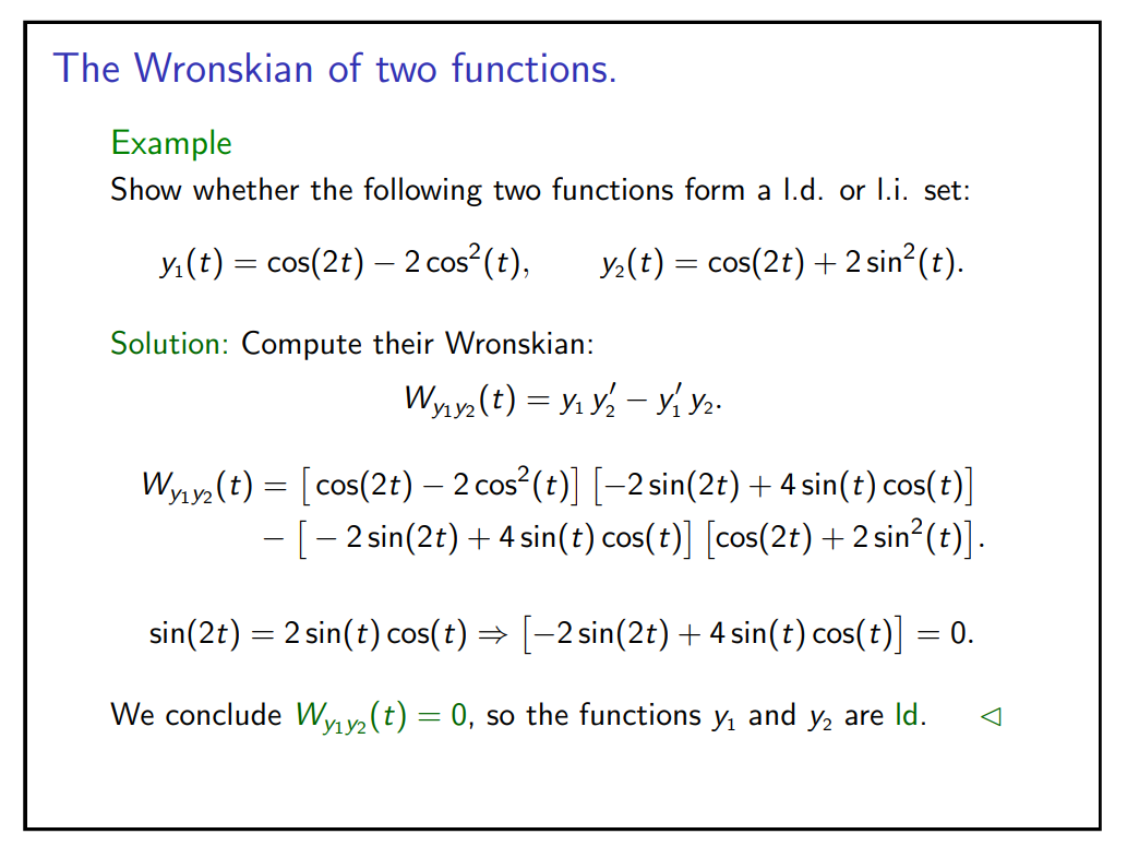
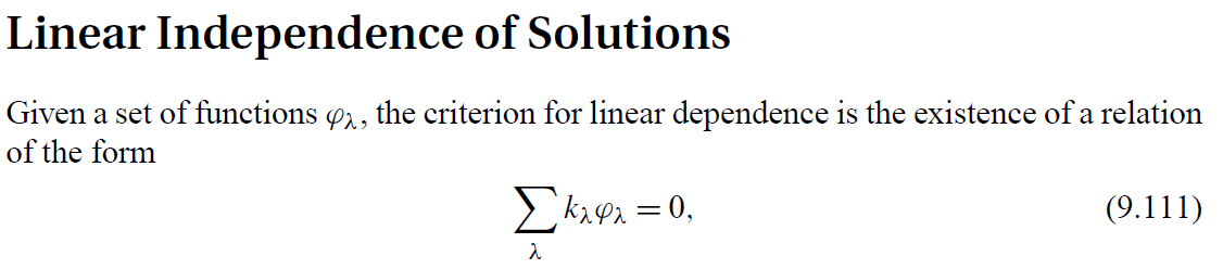
\text{{\color{red}The Wronskian of two functions}}
\text{The Wronskian of two functions } \displaystyle y_1, y_2: (t_1,t_2)\rightarrow \mathcal{R} \text{ is defined as}
W_{y_1y_2}(t)=y_1(t)y'_2(t)-y'_1(t)y_2(t)
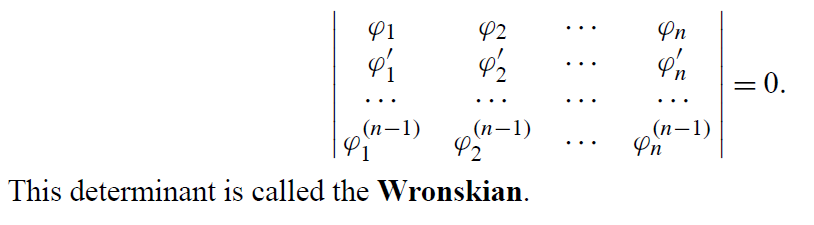
\text{It can also be seen as the determinant of the matrix }\displaystyle A(t)=\begin{bmatrix}
y_1 & y_2 \\
y'_1 &y'_2 \\
\end{bmatrix}
W_{y_1y_2}(t)=\text{det}\Big(A(t)\Big)
\begin{align*}
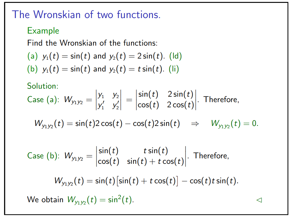
& \textbf{\textcolor{green}{Example:}} \quad \\
&\text{Show whether the following two functions form a linearly dependent (l.d.)}\\
&\text{or linearly independent (l.i.) set:} \\[6pt]
& y_1(t) = \cos(2t) - 2\cos^2(t), y_2(t) = \cos(2t) + 2\sin^2(t).
\end{align*}
\begin{align*}
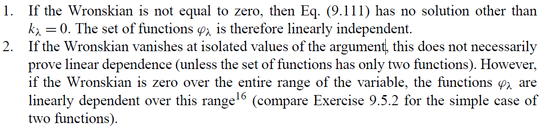
&\textbf{\textcolor{green}{Theorem (Wronskian and Linear Dependence).}} \quad\\
&\text{Let } y_1, y_2 : (t_1,t_2) \to \mathbb{R} \text{ be continuously differentiable functions.} \text{Then } y_1 \text{ and } y_2 \text{are linearly}\\
& \text{ dependent if and only if } \\
&\hspace{5cm}W_{y_1,y_2}(t) = 0 \quad \text{for all } t \in (t_1,t_2).
\end{align*}
For more problems, check:
https://tutorial.math.lamar.edu/classes/de/wronskian.aspx
\text{Abel's Theorem: if }y_1 \text{ and } y_2 \text { are any two solutions of the equation: }
y''+ P(x) y'+ Q(x) y=0
\text{where P, Q are continuous on an open interval I, then the Wronskian } W(y_1,y_2)(x) \text{ is given by}
\text{ {\color{red}Abel's Theorem} }
\text{Let us suppose that we know the solution }y_1 \text{ and we would like to find the second one } y_2
\text{The wronskian is either zero everywhere or nowhere zero}
\displaystyle W(x)=W(a) \exp \left[-\int_a^x P\left(x_1\right) d x_1\right] .
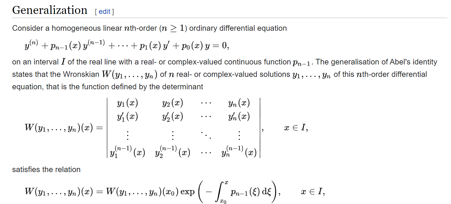
\displaystyle y_2(x)=y_1(x) \int^x \frac{\exp \left[-\displaystyle \int^{x_2} P\left(x_1\right) d x_1\right]}{\left[y_1\left(x_2\right)\right]^2} d x_2 .
\text{Let us suppose that we know the solution }y_1 \text{ and we would like to find the second one } y_2
\text{Proof}
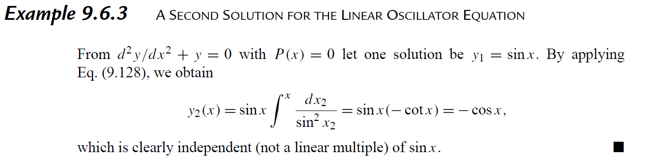
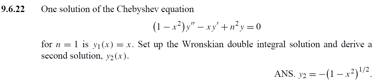
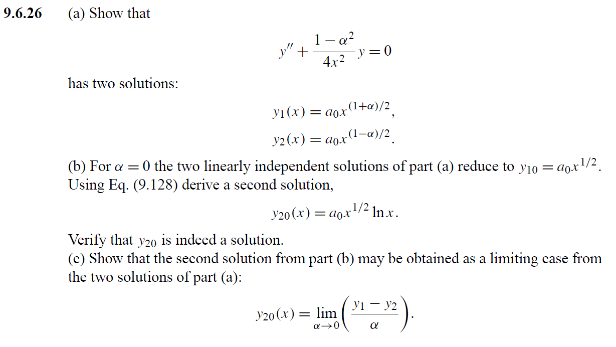
\text { If we have the important special case of } P(x)=0 \text {, }
y_2(x)=y_1(x) \int^x \frac{d x_2}{\left[y_1\left(x_2\right)\right]^2}
\begin{aligned}
y_2(x) & =y_1(x) \cdot\left(\frac{y_2(x)}{y_1(x)}\right)=y_1(x) \cdot \int^x\left(\frac{y_2(s)}{y_1(s)}\right)^{\prime} d s \\
& =y_1(x) \cdot \int^x \frac{y_2^{\prime}(s) y_1(s)-y_2(s) y_1^{\prime}(s)}{y_1^2(s)} d s=\int_1^x \frac{w(s)}{y_1^2(s)} d s \\
& =y_1(x) \cdot \int^x \frac{\exp ^{-\int^s P(t) d t}}{y_1^2(s)} d s
\end{aligned}
\text{Linear ODEs with constant coefficients}
\text{Consider the linear ODE with the form:}
y^{(n)}+a_{n-1}y^{(n-1)}+a_{(n-2)}y^{(n-2)}\dots +a_1y^\prime+a_0 y=0\hspace{1cm}\dots (1)
\text{Let us search solutions of the form: }
y(x)= e^{mx}
\displaystyle P(m)=m^n+a_{n-1}m^{n-1}+a_{(n-2)}m^{n-2}\dots +a_1 m+a_0=0
\text{By inserting this solution in Eq. 1, we get the following \color{purple}{caracterestic polynomials}:}
\text{This polynomial has n roots in the complex plane. If the root m is of multiplicity one, } e^{mx}
\text{is therefore one of the n {\color{purple}{independent solutions}} needed to get the general solution.}
\text{Case of higher multiplicity root:}
\text{Let us consider first the case of multiplicity 2: }m_0\text{ is adouble root}
\text{Let us suppose that the two roots are slightly different: }m_0, m_0+\delta
e^{m_0 x}, e^{(m_0+\delta) x} \text{are solutions of Eq. 1 and so is }\displaystyle \frac{e^{(m_0+\delta) x}-e^{m_0 x}}{\delta }
\text{The solutions of Eq.1 represent a cevtor space of dimension n. We need n \color{purple}{linearaly} }
\text{{\color{purple}{independent}} vector (solution), to represent the general solution}
\text{This basis is \color{purple}{not unique}}
y^{'''}-2 y^{''}+y^{'}-2y=0
\text{{\color{red}Problem}}\\
\text{Solve the following differential equation:}
\text{{\color{red}Solution:}}\\
\text{The caracterestic polynomial is:}\\
m^3-2m^2+m-2=0 \Rightarrow m^2(m-2)+m-2=0
\Rightarrow (m^2+1)(m-2)=0
\Rightarrow m=\pm i \text { or } m=2
\text{The general solution is therefore:}
y=Ae^{+i x}+B e^{-ix}+C e^{2x}
\text{It can also be expressed in terms of real functions:}
y=A^{'}\cos(x)+B^{'} \sin(x)+C e^{2x}
\text{Let us solve the following differential equation:}
y^{(4)}-2y^{(3)}+2y''-2y'+y=0
\text{{\color{red}Solution:}}
\text{The caracterestic polynomial for this equation is:}
m^4-2m^3+2m^2-2m+1=0 \Rightarrow (m^4+2m^2+1) -2m^3+-2m=0\\
\Rightarrow (m^2+1)^2 -2m(m^2+1)=0\\
\Rightarrow (m^2+1)(m-1)^2 =0\\
\text{The roots are: } i,-i \text{ and 1 (multiplicity 2)}
\text{The solution basis is: } e^{ix}, e^{-ix},e^{x}, xe^{x}
\text{{\color{red}Problem}}\\
y=Ae^{ix}+Be^{-ix}+Ce^{x}+Dxe^{x}
\text{Isobaric ODEs}
\text { An ODE } y^{\prime}=f(x, y) \text { is called \textcolor{purple}{isobaric} of degree } m \text { if }
f\left(t x, t^m y\right)=t^{m-1} f(x, y)
\text{If }m=1 \text{ then, it is called \textcolor{purple}{homogeneous}}
\text{Another way of defining the isobaric ODE is when} \displaystyle f(x,y)=\frac{M(x,y)}{N(x,y)}
y^{\prime}=f(x, y)\Rightarrow N(x,y)dy-M(x,y)dx=0
\text{Example:}
\displaystyle \frac{dy}{dx}=\frac{y-x}{y+x}
(y+x) dy-(y-x) dx=0
\Rightarrow
\text{Steps to solve isobaric ODEs}
1) \text{Check that the ODE is isobaric and find the corresponding }m
a) \text{ Using the definition: }f\left(t x, t^m y\right)=t^{m-1} f(x, y)
b) \text{ Using the form: }y^{\prime}=f(x, y)\Rightarrow N(x,y)dy-M(x,y)dx=0
\text{ in b) we give a weight } 1 \text{ for } x \text{ and a weight } m \text{ for y }
2) \text{After finding the weight } m\text{ that makes all the terms of equal weight, we do the change:}
y=x^m v
3) \text{Calculate }dy \text{ in terms of } dx \text{ and } dv \text{ and then solve the new ODE}
\text{Let us solve the following equation:}
\displaystyle \frac{dy}{dx}=\frac{y-x}{y+x}
\text{{\color{red}Solution:}}
\text{This equation can be rewritten as:}
(y+x) dy-(y-x) dx=0
\text{We will check if it is an isobaric equation:}
\text{ we give a weight 1 for x and m for y}
y dy
x dy
y dx
x dx
\text{weight}
2m
m+1
m+1
2
\text{{\color{red}Problem}}\\
\text{ All the terms will have the same weight if we put }m=1
\text{we put: } y=x^mv \text{, with } m=1
dy=v dx+x dv
\text{the equation becomes:}
(x+xv)(v dx+x dv)-(xv-x)dx=0
\displaystyle (1+v^2) dx+(1+v)xdv=0\Rightarrow \frac{dx}{x}+\frac{1+v}{1+v^2}dv=0
\displaystyle \Rightarrow \frac{dx}{x}+\frac{dv}{1+v^2}+\frac{vdv}{1+v^2}=0
\Rightarrow \ln(|x|)+\tan^{-1}(v)+\frac{1}{2}\ln(1+v^2)=cte
\Rightarrow \ln(|x|)+\tan^{-1}(y/x)+\frac{1}{2}\ln(1+(y/x)^2)=cte
\text{Example 2:}
\text{Solve the following ODE}
\displaystyle \frac{d y}{d x}=\frac{-\left(y^2+\frac{2}{x}\right)}{2 y x}
\displaystyle 2 yx d y+\left(y^2+\frac{2}{x}\right) dx=0
\text{Solution:}
\text{The equation can be written this way:}
2 yx d y
y^2 dx
\displaystyle \frac{2}{x} dx
\text{weight}
2m+1
2m+1
0
\text{In order to have the same weight, we need to have }m=-\frac{1}{2}
\text{we put }\displaystyle y=vx^{-\frac{1}{2}}=\frac{v}{\sqrt{x}}
\displaystyle dy=\frac{dv}{\sqrt{x}}-\frac{1}{2}v\frac{ dx }{\sqrt{x^3}}
\text{By injecting these result in the ODE, we get:}
\displaystyle vdv+\frac{dx}{x}=0
\text{The solution is therefore: }
\frac{1}{2}v^2+\ln(x)=c
\Rightarrow v=\pm \sqrt{-\ln(c^\prime x^2)}\Rightarrow y=\pm\sqrt{-\ln(c^\prime x^2)/x}
\text{{\color{red}Problem}}\\
\text{{\color{red}Nonhomogeneous second order ODE}}
y''+ P(x) y'+ Q(x) y=F(x)
\text{Let us consider the general form of the snd order ODE with a source term } F(x):
\text{The general solution has the form:}
\text{The particular solution }y_p(x) \text{ can be obtained as follows:}
\text{(for the proof, check the Petterson notes)}
y_1 \text { and } y_2 \text { are independent solutions of the {\textcolor{purple}{homogeneous}} equation. }
\displaystyle y_p(x)=y_2(x) \int^x \frac{y_1(s) F(s) d s}{W\left\{y_1(s), y_2(s)\right\}}-y_1(x) \int^x \frac{y_2(s) F(s) d s}{W\left\{y_1(s), y_2(s)\right\}}
\displaystyle y(x)=A y_1(x)+B y_2(x)+y_p(x)
\text{Example:}
\text { Let us solve the following non-homogeneous linear ODE: }
y^{\prime \prime}-3 {y^\prime}+2 y=x e^x
\text{The caracterestic polynomial is:}
r^2-3 r+2=0 \quad, \text{ and the roots are: } r=1,2
\text{The general solution is:}
y_1(x)=e^x, y_2(x)=e^{2 x}
\text { The homogeneous solutions is: }
\displaystyle y_{H}(x)=A e^x+B e^{2 x}
w(x)=\left|\begin{array}{ll}
e^x & e^{2 x} \\
e^x & 2 e^{2 x}
\end{array}\right|=e^{3 x}
\displaystyle y_p(x)=e^{2 x} \cdot \int^x e^s s e^s e^{-3 s} d s-e^x \int^x e^{2 s} s e^s e^{-3 s} d s
=-(1+x+\frac{x^2}{2} )e^x
\displaystyle y(x)=A e^x+B e^{2 x}-(1+x+\frac{x^2}{2} )e^x
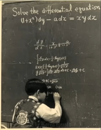
\text{Can you find what is the solution of this kid?}
Ordinary differential equations
By smstry


