Lecture 10 : Principal Component Analysis (PCA)
Assoc. Prof. Yuan-Sen Ting
Astron 5550 : Advanced Astronomical Data Analysis
Logistics
Select and submit your topic for group project 2 (on Carmen), by this Friday, 11:59pm
Plan for Today :
Principal Component Analysis
Eigenvectors, Eigenvalues
Lagrange Multipliers
Singular Value Decomposition (SVD)
Unsupervised Learning in Astronomy
Supervised learning maps input \( x \) to output \( y \) with specific target variables
Unsupervised learning reveals inherent data structure of \( x \) without explicit target variables
Two main unsupervised tasks: dimension reduction and clustering
Unsupervised methods particularly valuable in astronomy for understanding complex datasets
Introduction to Dimension Reduction
High-dimensional astronomical data (spectra, images, time series) requires compression for interpretation
Dimension reduction projects data from high-dimensional space to lower-dimensional manifolds
PCA aims to compress/decompress data while preserving essential information
Visual understanding of high-dimensional data becomes possible through effective dimension reduction

First paper !
Physical Motivation for Dimension Reduction
Astrophysical processes are governed by finite latent variables despite high-dimensional observations
Stellar chemical abundances show correlations through common nucleosynthesis processes
Quasar spectra complexity stems from few physical parameters (accretion rate, viewing angle, redshift)
Benefits include computational efficiency and improved data transmission for space missions
Data as Realizations of a Probability Distribution
Observed data points can be viewed as realizations from an unknown probability distribution \( P(X) \)
Assumption: observations are independent and identically distributed (I.I.D.) samples
Dataset consists of I.I.D. samples \( \mathcal{X} = \{\mathbf{x}_1, ..., \mathbf{x}_n\} \), where each \( \mathbf{x}_i \in \mathbb{R}^D \) is a \( D \)-dimensional vector
Dimension reduction asks: does \( P(X) \) live on a lower-dimensional manifold?
Principal Component Analysis: A Dual Perspective
PCA finds a orthogonal lower-dimensional projection \( \mathbf{z} \in \mathbb{R}^M \) of data \( \mathbf{x} \in \mathbb{R}^D \) where \( M < D \)
We assume data is centered with zero mean:
\( E[\mathbf{x}] = \bar{\mathbf{x}} \simeq \frac{1}{N}\sum_{i=1}^N \mathbf{x}_i = \mathbf{0} \), by centering the data
Variance Maximization: Find directions of maximum variance in high-dimensional space
Reconstruction Error Minimization: Minimize squared error between original data and reconstruction
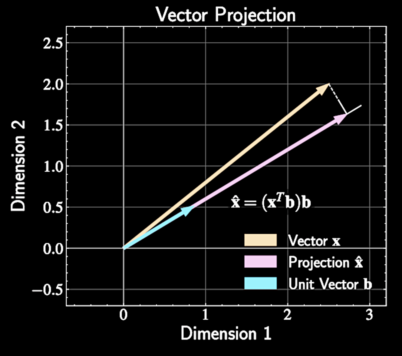
Vector Projection Fundamentals
Vector projection of \( \mathbf{x} \) onto unit vector \( \mathbf{b} \) is given by
Scalar term \( \mathbf{x}^T \mathbf{b} \) measures how much of vector \( \mathbf{x} \) points in direction \( \mathbf{b} \)
Vector can be decomposed using orthonormal basis:
\widehat{\mathbf{x}} = (\mathbf{x}^T \mathbf{b})\mathbf{b}
\mathbf{x} = \sum_{d=1}^D (\mathbf{x} \cdot \mathbf{b}_d )\mathbf{b}_d
Vector Projection Fundamentals
PCA aims to find orthonormal \( {\mathbf{b}_1, \mathbf{b}_2, ..., \mathbf{b}_M} \) where \( M < D \)
First sum represents low-dimensional approximation;
second sum contains residual components
Data vector decomposition:
\mathbf{x} = \sum_{m=1}^M (\mathbf{x} \cdot \mathbf{b}_m)\mathbf{b}_m + \sum_{j=M+1}^D (\mathbf{x} \cdot \mathbf{b}_j)\mathbf{b}_j
Vector Projection Fundamentals
Coefficient vectors:
Basis :
Matrix formulation with basis vectors:
\mathbf{B}_M = [\mathbf{b}_1, \mathbf{b}_2, \ldots, \mathbf{b}_M]
\mathbf{B}_R = [\mathbf{b}_{M+1}, \mathbf{b}_{M+2}, \ldots, \mathbf{b}_D]
\mathbf{x} = \mathbf{B}_M\mathbf{z}_M + \mathbf{B}_R\mathbf{z}_R
\mathbf{z}_M = [\mathbf{x}^T \mathbf{b}_1, \mathbf{x}^T \mathbf{b}_2, \ldots, \mathbf{x}^T \mathbf{b}_M]^T
\mathbf{z}_R = [\mathbf{x}^T \mathbf{b}_{M+1}, \ldots, \mathbf{x}^T \mathbf{b}_D]^T
Orthonormal Basis Representation
Data vector in orthonormal basis:
Total variance in coefficient space:
\mathbf{x} = \sum_{m=1}^D z_m\mathbf{b}_m, \quad z_m = \mathbf{x}^T \mathbf{b}_m
\text{Total Variance} = E[\mathbf{x}^2] = E\left[\left|\sum_{m=1}^D z_m\mathbf{b}_m\right|^2\right] = E \left[\sum_{m=1}^D z_m^2\right]
Variance Decomposition and Reconstruction Error
Total variance can be split into two components:
First term: variance captured by \( M \) principal components
Second term: variance in remaining directions = reconstruction error
\text{Total Variance} = E \left[\sum_{m=1}^D z_m^2\right] = E \left[\sum_{m=1}^M z_m^2\right] + E \left[\sum_{j=M+1}^D z_j^2\right]
PCA finds directions of maximum variance and optimal low-dimensional approximation
PCA Optimization Framework
PCA seeks basis vectors \( \mathbf{b}_1, ..., \mathbf{b}_M \) that maximize variance while maintaining orthonormality
Let's find the first component.
Projections are defined as
\text{Var}[z_1] = \frac{1}{N} \sum_{n=1}^N z_{1n}^2
z_{1n} = \mathbf{x}_n^T \mathbf{b}_1 = \mathbf{b}_1^T\mathbf{x}_n
Linear Transformations and Covariance
For linear transformation of random vector \( \mathbf{Y} = \mathbf{A}\mathbf{X} \), covariance transforms as:
For scalar projection \( z_1 = \mathbf{b}_1^T\mathbf{x} \), variance is
\text{Cov}(\mathbf{Y}) = \mathbf{A} \cdot \text{Cov}(\mathbf{X}) \cdot \mathbf{A}^T
\text{Var}[z_1] = \mathbf{b}_1^T \cdot \text{Cov}(\mathbf{x}) \cdot \mathbf{b}_1 \equiv \mathbf{b}_1^T \mathbf{S} \mathbf{b}_1
Linear Transformations and Covariance
Without constraints, optimization is ill-defined: scaling \( \mathbf{b}_1 \) by constant \( c > 1 \) gives variance \( \text{Var}[z_1'] = c^2 \mathbf{b}_1^T \mathbf{S} \mathbf{b}_1 = c^2 \text{Var}[z_1] \)
Could make variance arbitrarily large by increasing magnitude of \( \mathbf{b}_1 \)
Only direction of \( \mathbf{b}_1 \) matters, not its magnitude
Need to constrain \( \mathbf{b}_1 \) to be a unit vector: \( |\mathbf{b}_1|^2 = \mathbf{b}_1^T\mathbf{b}_1 = 1 \)
Constrained Optimization Problem
First principal component formulated as:
This is a constrained optimization problem common in physics
\max_{\mathbf{b}_1} \mathbf{b}_1^T \mathbf{S} \mathbf{b}_1 \quad \text{subject to} \quad \mathbf{b}_1^T\mathbf{b}_1 = 1
Introduction to Lagrange Multipliers
Lagrange multipliers solve constrained optimization problems: finding extrema of \( f(x) \) subject to constraint \( g(x) = 0 \)
Unconstrained optimization finds extrema where gradient equals zero: \( \nabla f(x) = 0 \)
Constrained optimization restricts search to points
that satisfy \( g(x) = 0 \)
PCA constraint is \( g(\mathbf{b}_1) = \mathbf{b}_1^T\mathbf{b}_1 - 1 = 0 \).
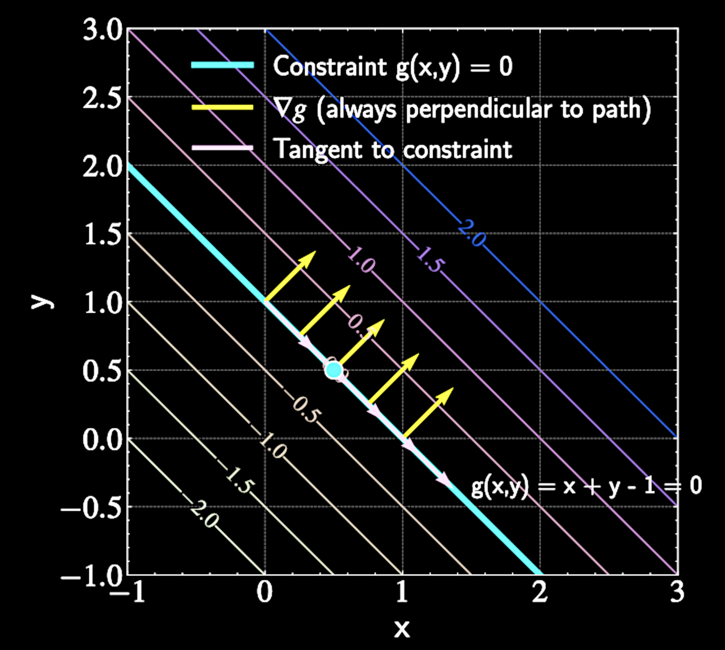
Geometric Intuition
At constrained extremum, moving along constraint path shouldn't improve the function
Gradient \( \nabla f \) must be perpendicular to constraint path at extrema points
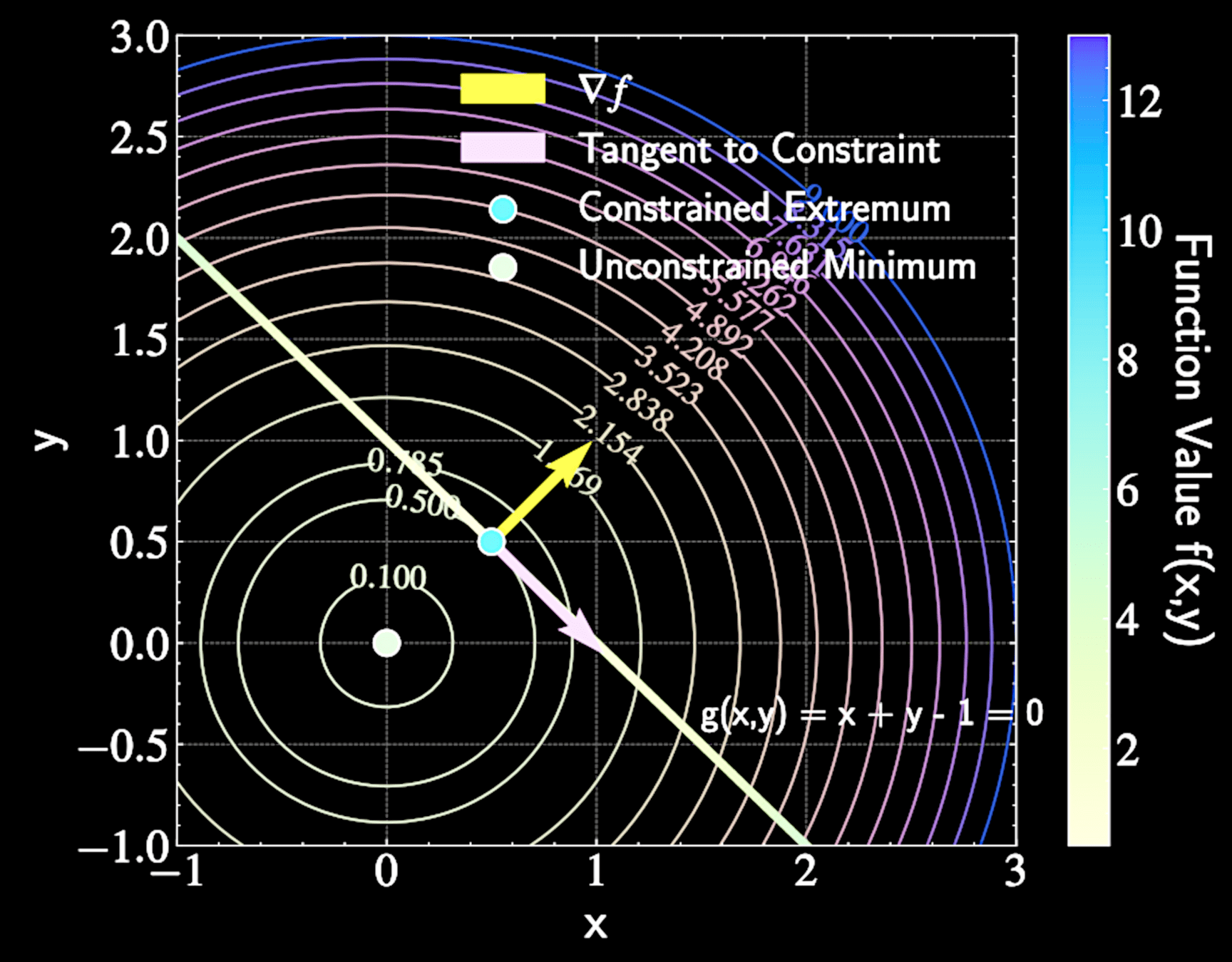
f(x,y) = x^2 + y^2
Geometric Intuition
At constrained maximum, moving along constraint path shouldn't improve the function
Gradient \( \nabla f \) must be perpendicular to constraint path at extrema points
Gradient of constraint \( \nabla g \) is always perpendicular to constraint path
The Lagrangian Function
Mathematically: \( \nabla f(x) = \lambda \nabla g(x) \), where \( \lambda \): Lagrange multiplier
Note: this is a necessary (but not sufficient) condition for finding constrained extrema
Introduces Lagrangian function:
\mathcal{L}(x, \lambda) = f(x) - \lambda g(x)
At constrained extremum, gradients of \( f \) and \( g \) must be parallel to each other
Finding Critical Points
Take partial derivatives with respect to \( x \) and set to zero:
Recover the necessary condition
Taking derivative with respect to \( \lambda \):
\frac{\partial \mathcal{L}}{\partial \lambda} = -g(x) = 0 \Rightarrow g(x) = 0
\nabla_x \mathcal{L} = \nabla f(x) - \lambda \nabla g(x) = 0
\nabla f(x) = \lambda \nabla g(x)
f(x,y) = x^2 + y^2
Example Application
Find minimum value of
With Lagrange multiplier:
\mathcal{L}(x,y,\lambda) = x^2 + y^2 - \lambda(x + y - 1)
f(x,y) = x^2 + y^2
subject to constraint
g(x,y) = x + y - 1 = 0
Example Application
Partial derivatives:
x = y = \frac{\lambda}{2}
\frac{\partial \mathcal{L}}{\partial x} = 2x - \lambda = 0
\Rightarrow x = \frac{\lambda}{2}
\frac{\partial \mathcal{L}}{\partial y} = 2y - \lambda = 0
\Rightarrow y = \frac{\lambda}{2}
Example Application
Constraint equation:
\frac{\partial \mathcal{L}}{\partial \lambda} = -(x + y - 1) = 0
\Rightarrow x + y = 1
\Rightarrow x = y = \frac{1}{2}
Minimum value:
f\left(\frac{1}{2}, \frac{1}{2}\right) = \left(\frac{1}{2}\right)^2 + \left(\frac{1}{2}\right)^2 = \frac{1}{2}
f(x,y) = x^2 + y^2
Extension to Multiple Constraints
For constraints \( g_1(x) = 0, g_2(x) = 0, ..., g_m(x) = 0 \), condition becomes:
Geometric interpretation: \( \nabla f(x) \) must be perpendicular to the surface spanned by the multiple gradient directions
\nabla f(x) = \lambda_1 \nabla g_1(x) + \lambda_2 \nabla g_2(x) + ... + \lambda_m \nabla g_m(x)
\mathcal{L}(x, \lambda_1, ..., \lambda_m) = f(x) - \lambda_1 g_1(x) - ... - \lambda_m g_m(x)
PCA as a Constrained Optimization Problem
Objective: Maximize variance of projected data subject to unit vector constraint
Mathematical formulation:
\max_{\mathbf{b}_1} \mathbf{b}_1^T \mathbf{S} \mathbf{b}_1 \quad \text{subject to} \quad \mathbf{b}_1^T\mathbf{b}_1 = 1
Applying Lagrange multipliers
\mathcal{L}(\mathbf{b}_1, \lambda_1) = \mathbf{b}_1^T \mathbf{S} \mathbf{b}_1 - \lambda_1(\mathbf{b}_1^T\mathbf{b}_1 - 1)
Computing Critical Points
Differentiate with respect to \( \lambda_1 \):
Yields original constraint: \( \mathbf{b}_1^T\mathbf{b}_1 = 1 \)
\frac{\partial\mathcal{L}}{\partial\lambda_1} = -(\mathbf{b}_1^T\mathbf{b}_1 - 1) = 0
Differentiate with respect to \( \mathbf{b}_1 \):
\frac{\partial\mathcal{L}}{\partial \mathbf{b}_1} = 2 \mathbf{S} \mathbf{b}_1 - 2\lambda_1\mathbf{b}_1 = 0
\Rightarrow \mathbf{S} \mathbf{b}_1 = \lambda_1\mathbf{b}_1
Computing Critical Points
Equation \( \mathbf{S} \mathbf{b}_1 = \lambda_1\mathbf{b}_1 \) is an eigenvector equation
\( \mathbf{b}_1 \) must be an eigenvector of covariance matrix \( \mathbf{S} \)
\( \lambda_1 \) is the corresponding eigenvalue
Eigenvectors maintain their direction under transformation, with scale factor equal to eigenvalue
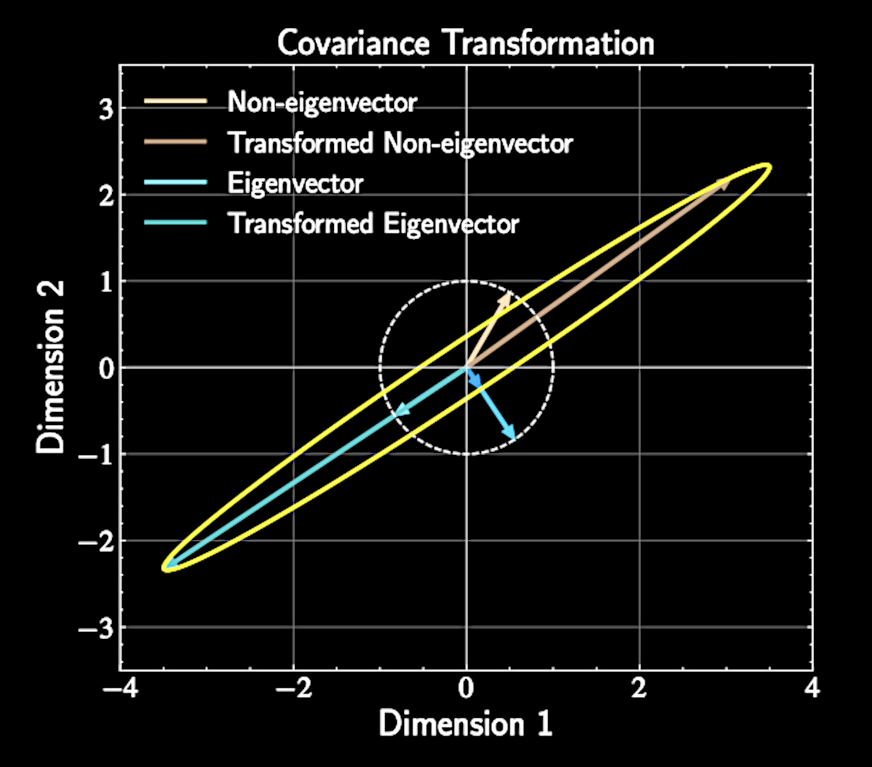
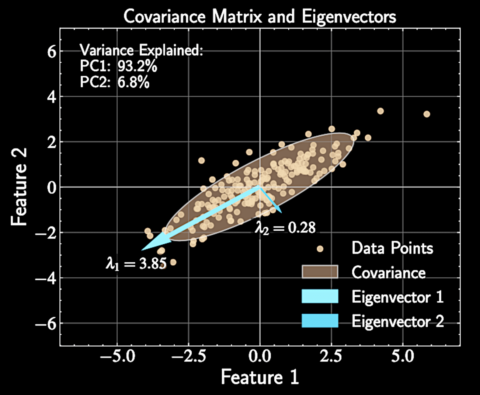
Geometric Interpretation of Eigenvectors
Covariance matrix describes how data "stretches" in different directions
Eigenvectors represent principal axes of this stretching
Eigenvalues tell us how much stretching occurs along each axis
Principal components align with natural axes of variation in the data
Connecting Eigenvalues to Variance
Variance of projected data equals: \( \text{Var}[z_1] = \mathbf{b}_1^T \mathbf{S} \mathbf{b}_1 \)
Substituting eigenvector relationship:
Variance when projecting onto eigenvector equals corresponding eigenvalue
First principal component = eigenvector with largest eigenvalue
\text{Var}[z_1] = \mathbf{b}_1^T(\lambda_1\mathbf{b}_1) = \lambda_1\mathbf{b}_1^T\mathbf{b}_1 = \lambda_1
Finding Higher-Order Principal Components
First principal component captures maximum variance, but additional components needed for effective dimension reduction
Second principal component must: 1) capture maximum remaining variance and 2) be orthogonal to first component (inductive bias)
Mathematical formulation:
\max_{\mathbf{b}_2} \mathbf{b}_2^T \mathbf{S} \mathbf{b}_2 \quad \text{subject to} \quad \mathbf{b}_2^T\mathbf{b}_2 = 1 \quad \text{and} \quad \mathbf{b}_1^T\mathbf{b}_2 = 0
Lagrangian with Multiple Constraints
Introduce two Lagrange multipliers for two constraints.
Lagrangian function:
Differentiate with respect to \( \mathbf{b}_2 \):
\mathcal{L}(\mathbf{b}_2, \lambda_2, \mu) = \mathbf{b}_2^T \mathbf{S} \mathbf{b}_2 - \lambda_2(\mathbf{b}_2^T\mathbf{b}_2 - 1) - \mu(\mathbf{b}_1^T\mathbf{b}_2)
\frac{\partial\mathcal{L}}{\partial \mathbf{b}_2} = 2 \mathbf{S} \mathbf{b}_2 - 2\lambda_2\mathbf{b}_2 - \mu\mathbf{b}_1 = 0
Solving for the Second Component
Multiply derivative equation by \( \mathbf{b}_1^T \)
Since \( \mathbf{b}_1^T \mathbf{S} = \lambda_1\mathbf{b}_1^T \) and \( \mathbf{b}_1^T\mathbf{b}_2 = 0 \), we get \( \mu = 0 \)
2\mathbf{b}_1^T \mathbf{S} \mathbf{b}_2 - \mu = 0
Substituting back:
\mathbf{S} \mathbf{b}_2 = \lambda_2\mathbf{b}_2
2 \mathbf{S} \mathbf{b}_2 - 2\lambda_2\mathbf{b}_2 - \mu\mathbf{b}_1 = 0
Second Principal Component is an Eigenvector
Second principal component \( \mathbf{b}_2 \) is also an eigenvector of covariance matrix \( \mathbf{S} \)
Due to orthogonality constraint, it must be a different eigenvector than \( \mathbf{b}_1 \)
Variance captured by \( \mathbf{b}_2 \) equals eigenvalue \( \lambda_2 \)
To maximize variance, choose eigenvector with second largest eigenvalue
Mathematical Induction for PCA
Need rigorous proof that \( m \)-th principal component corresponds to \( m \)-th largest eigenvalue
Mathematical induction provides elegant proof without repetitive calculations
Base case the inductive step
Like domino effect: prove first case and that each case implies the next
Setting Up the Induction
Base case: First principal component \( \mathbf{b}_1 \) is eigenvector with largest eigenvalue \( \lambda_1 \) (already proven)
Inductive step: Prove \( M \)-th principal component is eigenvector with \( M \)-th largest eigenvalue \( \lambda_M \), if the other \( M-1 \) were already true
Key insight: \( M \)-th component maximizes variance in residual data after removing first \( M-1 \) components
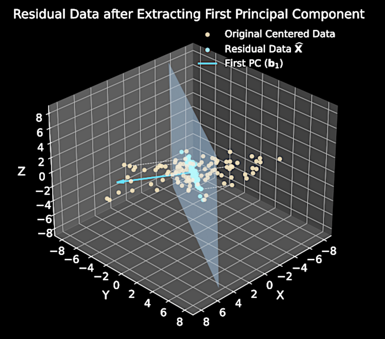
Residual Data Analysis
Original data matrix: \( \mathbf{X} \in \mathbb{R}^{N \times D} \) (each row is a data point)
Projection onto first \( M-1 \) principal components:
Residual data:
\sum_{m=1}^{M-1} \mathbf{X}\mathbf{b}_m\mathbf{b}_m^T
\widehat{\mathbf{X}} = \mathbf{X} - \sum_{m=1}^{M-1} \mathbf{X}\mathbf{b}_m\mathbf{b}_m^T
Residual Data Analysis
Matrix form:
Residual data covariance:
\widehat{\mathbf{X}} = \mathbf{X} - \mathbf{X}\mathbf{B}_{M-1}\mathbf{B}_{M-1}^T \quad \text{where} \; \mathbf{B}_{m-1} = [\mathbf{b}_1, \mathbf{b}_2, ..., \mathbf{b}_{m-1}]
\widehat{\mathbf{S}} = \frac{1}{N}\widehat{\mathbf{X}}^T\widehat{\mathbf{X}}
Covariance of Residual Data
Expanding expression:
Original covariance:
\widehat{\mathbf{S}} = \frac{1}{N}(\mathbf{X} - \mathbf{X}\mathbf{B}_{M-1}\mathbf{B}_{M-1}^T)^T(\mathbf{X} - \mathbf{X}\mathbf{B}_{M-1}\mathbf{B}_{M-1}^T)
\mathbf{S} = \frac{1}{N}\mathbf{X}^T \mathbf{X}
Substituting:
\widehat{\mathbf{S}} = \mathbf{S} - \mathbf{S}\mathbf{B}_{M-1}\mathbf{B}_{M-1}^T - \mathbf{B}_{M-1}\mathbf{B}_{M-1}^T \mathbf{S} + \mathbf{B}_{M-1}\mathbf{B}_{M-1}^T \mathbf{S} \mathbf{B}_{M-1}\mathbf{B}_{M-1}^T
Simplified Residual Covariance
For eigenvectors: \( \mathbf{S}\mathbf{b}_i = \lambda_i\mathbf{b}_i \) for \( i = 1, 2, \ldots, m-1\)
Matrix form: \( \mathbf{S}\mathbf{B}_{M-1} = \mathbf{B}_{M-1}\mathbf{\Lambda}_{M-1} \) and \( \mathbf{B}_{M-1}^T\mathbf{S} = \mathbf{\Lambda}_{M-1}\mathbf{B}_{M-1}^T \) where \( \mathbf{\Lambda}_{M-1}\) contains eigenvalues
Orthonormality gives:
\widehat{\mathbf{S}} = \mathbf{S} - \mathbf{S}\mathbf{B}_{M-1}\mathbf{B}_{M-1}^T - \mathbf{B}_{M-1}\mathbf{B}_{M-1}^T \mathbf{S} + \mathbf{B}_{M-1}\mathbf{B}_{M-1}^T \mathbf{S} \mathbf{B}_{M-1}\mathbf{B}_{M-1}^T
\mathbf{B}_{M-1}^T \mathbf{B}_{M-1} = \mathbf{I}_{M-1}
Simplified Residual Covariance
Substituting eigenvector properties:
Expanded form:
Residual covariance equals original covariance minus variance explained by first \( M-1 \) components
\widehat{\mathbf{S}} = \mathbf{S} - \mathbf{B}_{M-1}\mathbf{\Lambda}_{M-1}\mathbf{B}_{M-1}^T
\widehat{\mathbf{S}} = \mathbf{S} - \sum_{m=1}^{M-1} \lambda_m \mathbf{b}_m\mathbf{b}_m^T
Effect on Previous Eigenvectors
For any previous eigenvectors \( \mathbf{b}_k \) where \( k < M \):
Using \( \mathbf{S}\mathbf{b}_k = \lambda_k\mathbf{b}_k \) and orthonormality:
First \( M-1 \) eigenvectors become eigenvectors of \( \widehat{\mathbf{S}} \) with eigenvalue 0
\widehat{\mathbf{S}}\mathbf{b}_k = \mathbf{S}\mathbf{b}_k - \sum_{m=1}^{M-1} \lambda_m \mathbf{b}_m\mathbf{b}_m^T\mathbf{b}_k
\widehat{\mathbf{S}}\mathbf{b}_k = \lambda_k\mathbf{b}_k - \lambda_k \mathbf{b}_k = 0
Effect on Previous Eigenvectors
For the remaining eigenvectors \( \mathbf{b}_j \) where \( j \geq M \):
Using \( \mathbf{S}\mathbf{b}_j = \lambda_j\mathbf{b}_j \) and orthonormality:
\( \mathbf{b}_j\) remains an eigenvector of \(\widehat{\mathbf{S}}\) with the same eigenvalue \(\lambda_j\) for all \(j \geq M\).
\widehat{\mathbf{S}}\mathbf{b}_j = \mathbf{S}\mathbf{b}_j - \sum_{m=1}^{M-1} \lambda_m \mathbf{b}_m\mathbf{b}_m^T\mathbf{b}_j
\widehat{\mathbf{S}}\mathbf{b}_j = \lambda_j\mathbf{b}_j
Eigenvalue Spectrum and Maximum Variance
Eigenvalue spectrum of \( \widehat{\mathbf{S}} \): \( \{0, 0, \ldots, 0, \lambda_M, \lambda_{M+1}, \ldots, \lambda_D \} \)
First \( M-1 \) eigenvalues are zero (corresponding to \( \mathbf{b}_1, \mathbf{b}_2, \ldots, \mathbf{b}_{m-1} \))
Without loss of generality, assuming \( \lambda_M \geq \lambda_{M+1} \geq ... \geq \lambda_D \), largest eigenvalue of \( \widehat{\mathbf{S}} \) is \( \lambda_M \)
Corresponding eigenvector is \( \mathbf{b}_M \) - this maximizes variance in residual data
Completing the Induction Proof
We've shown \( M \)-th principal component is eigenvector \( \mathbf{b}_M \) with \( M \)-th largest eigenvalue \( \lambda_M \)
This completes the inductive step: if statement holds for first \( M-1 \) components, it holds for \( M \)-th component
By mathematical induction, all principal components are eigenvectors of covariance matrix in order of decreasing eigenvalues
Practical implication: Compute eigendecomposition once, select components in order of decreasing eigenvalues
Basic Implementation of PCA
Center data matrix \( \mathbf{X} \)
Calculate covariance \( \mathbf{S} = \frac{1}{N}\mathbf{X}^T \mathbf{X} \)
Compute eigendecomposition, sort eigenvectors by eigenvalues,
Select first \( M \) eigenvectors, project data onto new basis
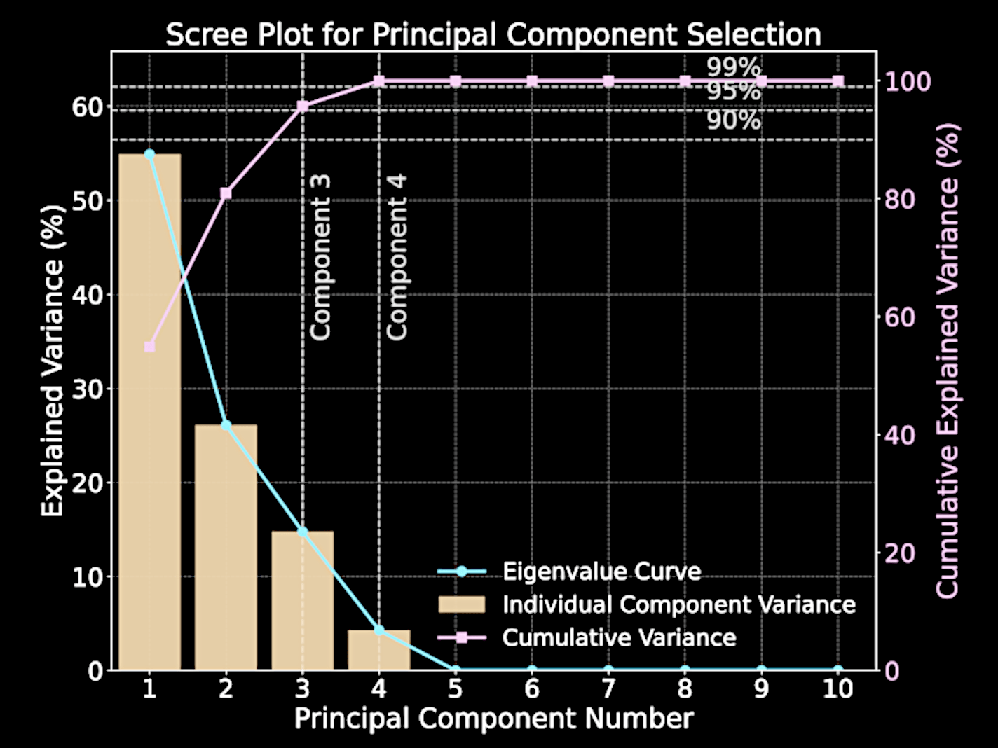
Selecting Number of Components
Variance captured by \( m \)-th principal component equals corresponding eigenvalue \( \lambda_m \)
Total variance: \( \sum_{m=1}^D \lambda_m \); Captured variance with \( M \) components: \( \sum_{m=1}^M \lambda_i \)
Explained variance ratio:
Scree plot visualizes eigenvalues versus their indices; "elbow" indicates natural cutoff point
\frac{\sum_{m=1}^M \lambda_i}{\sum_{m=1}^D \lambda_i}
Computational Challenges of Standard PCA
Diagonalizing \(D \times D\) covariance matrix has complexity \(\mathcal{O}(D^3)\)
Astronomical data often has thousands to tens of thousands of dimensions (spectra, images, time series)
Example: 10,000 wavelength bins requires \(\sim 10^{12} \) operations
Standard approach becomes computationally infeasible for datasets with a large number of input dimensions
Singular Value Decomposition (SVD)
Any real matrix \(\mathbf{X} \in \mathbb{R}^{N \times D}\) can be factorized as
\(\mathbf{U} \in \mathbb{R}^{N \times N}\): column orthonormal matrix
\(\mathbf{\Sigma} \in \mathbb{R}^{N \times D}\): diagonal matrix of "singular values" \(\sigma_i \)
\(\mathbf{V} \in \mathbb{R}^{D \times D}\): row orthonormal matrix
\mathbf{X} = \mathbf{U\Sigma V}^T
Geometric Interpretation of SVD
SVD decomposes a linear transformation into three operations
Rotation/reflection in output space via matrix \(\mathbf{U}\)
Scaling along coordinate axes via matrix \(\mathbf{\Sigma}\)
Rotation/reflection in input space via matrix \(\mathbf{V}^T\)
\mathbf{X} = \mathbf{U\Sigma V}^T
Computational Advantages of SVD
SVD complexity: \(\mathcal{O}(\min(ND^2, N^2D))\) vs. PCA's \(\mathcal{O}(D^3)\)
For \(N < D\): complexity becomes \(\mathcal{O}(N^2D)\)
Example: 100 samples × 10,000 features: \(\mathcal{O}(10^8)\) vs \(\mathcal{O}(10^{12})\)
Four orders of magnitude faster - days reduced to seconds
\mathbf{X} = \mathbf{U\Sigma V}^T
Connecting SVD to PCA
PCA's covariance matrix: \(\mathbf{S} = \frac{1}{N}\mathbf{X}^T\mathbf{X}\)
Substituting SVD:
Since \(\mathbf{U}^T\mathbf{U} = \mathbf{I}\):
This is the eigendecomposition of \(\mathbf{S}\)!
\mathbf{X} = \mathbf{U\Sigma V}^T
\mathbf{S} = \frac{1}{N}\mathbf{V\Sigma}^T\mathbf{U}^T\mathbf{U\Sigma V}^T
\mathbf{S} = \mathbf{V}\left(\frac{1}{N}\mathbf{\Sigma}^T\mathbf{\Sigma}\right)\mathbf{V}^T
SVD-PCA Equivalence
Columns of \(\mathbf{V}\) are eigenvectors of \(\mathbf{S}\) (our principal components)
Eigenvalues of \(\mathbf{S}\) equal \(\sigma_i^2/N\), where \(\sigma_i\) are singular values
SVD gives us PCA results without forming the covariance matrix
Avoids both computational complexity and numerical instability
Implementing PCA via SVD
Center the data matrix \(\mathbf{X}\)
Compute SVD: \(\mathbf{X} = \mathbf{U\Sigma V}^T\)
Use rows of \(\mathbf{V}\) as eigenvectors, \( \frac{1}{N} \Sigma^T \Sigma \) as eigenvalues.
Sort eigenvectors by eigenvalues, select first \( M \) eigenvectors,
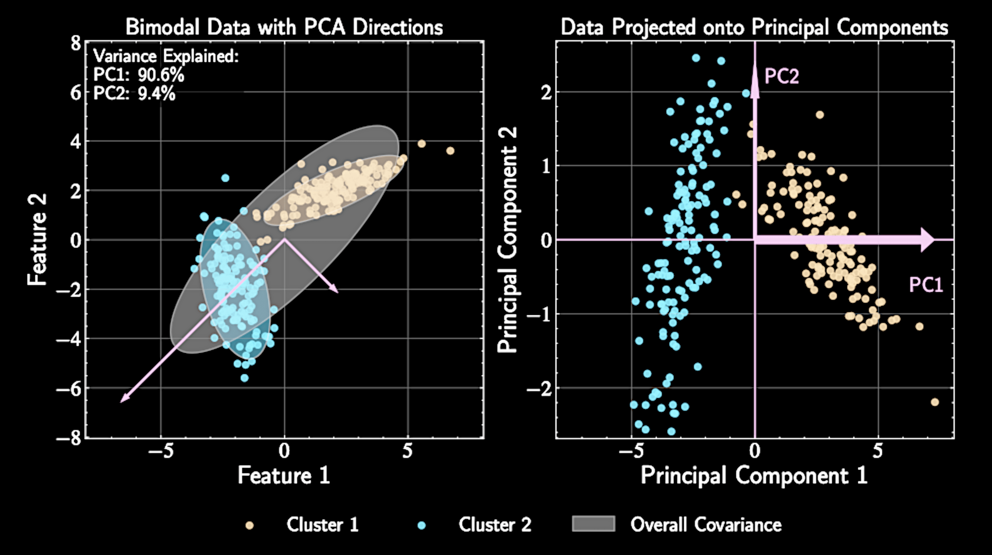
Limitations of Principal Component Analysis
Orthogonality constraint rarely matches physical reality
Principal components may mix multiple physical processes
First PC maximizes variance, not necessarily physical interpretability
PCA also assumes that the data forms a "blob". Data with multiple modes makes PCA less interpretable / useful.
Beyond Principal Component Analysis
Independent Component Analysis (ICA) maximizes statistical independence, instead of using covariance
ICA can better separate physically independent sources
Neural network autoencoders provide nonlinear generalizations
Advanced methods trade simplicity for more realistic modeling
What we have learned:
Principal Component Analysis
Eigenvectors, Eigenvalues
Lagrange Multipliers
Singular Value Decomposition (SVD)
Astron 5550 - Lecture 10
By Yuan-Sen Ting


