Lecture 13 : Markov Chain Monte Carlo

Assoc. Prof. Yuan-Sen Ting

Astron 5550 : Advanced Astronomical Data Analysis

Logistics

Homework Assignment 4 due this Friday,11:59pm

Group Project 2 - Presentation - April 16 (next Wednesday)

Group Project 2 - Report - April 28 (no deferment)

Logistics

Homework Assignment 4 due this Friday,11:59pm

Group Project 2 - Presentation - April 16 (next Wednesday)

Group Project 2 - Report - April 28 (no deferment)

Plan for Today :

Detailed Balance

Ergodicity

Convergence Test, Autocorrelation and Effective Sample Size

Metropolis-Hasting Algorithms and Gibbs Sampling

Limitations of Basic Sampling Methods

Inverse CDF transform sampling rarely works for complex astronomical posteriors

Rejection sampling efficiency drops dramatically in high-dimensional spaces

Astronomical posteriors feature multiple modes, correlated parameters, and irregular geometries

Bayesian methods characterize full posterior distributions beyond "best-fit" parameters

Understanding Markov Chains

Markov chain: like a traveler exploring Columbus using only current location to decide next stop

Each step depends only on current state, not the history of previously visited locations

States represent points in parameter space of our models

P(X_{t+1} = x | X_0 = x_0, X_1 = x_1, ..., X_t = x_t)

= P(X_{t+1} = x | X_t = x_t)

Understanding Markov Chains

Transition matrix \(T(\mathbf{x}, \mathbf{x'})\) is like a traveler's guidebook suggesting where to go next

Specifies probability of moving from current location \(\mathbf{x}\) to next location \(\mathbf{x'}\)

Understanding Markov Chains

Transition matrix \(T(\mathbf{x}, \mathbf{x'})\) is like a traveler's guidebook suggesting where to go next

Specifies probability of moving from current location \(\mathbf{x}\) to next location \(\mathbf{x'}\)

Guidebook directing traveler between neighborhoods of Columbus

Goal: design a guidebook that makes visitation pattern follow population distribution

Stationary Distributions

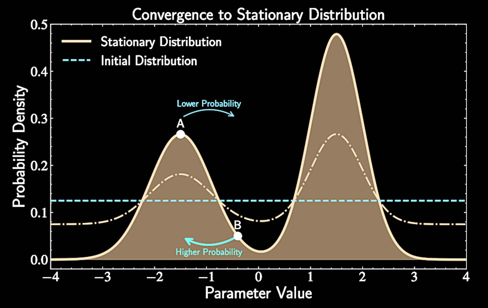
Once traveler's exploration pattern matches population distribution, it stays that way

The "equilibrium" end point of a Markov Chain

Stationary distribution: if traveler follows population distribution, they'll continue to do so

p(\mathbf{x'}) = \int p(\mathbf{x}) T(\mathbf{x}, \mathbf{x'}) d\mathbf{x} \equiv (Tp)(\mathbf{x})

Understanding Markov Chain Monte Carlo

We can design guidebooks (transition matrix) making posterior distribution the stationary distribution

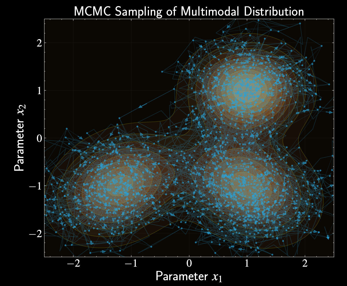
Creates random walk where walker spends time in regions proportional to posterior probability

After enough exploration, each footstep of the traveler becomes a sample from our posterior

Detailed Balance

Key question: How do we guarantee our target (posterior) distribution \( p (\mathbf{x} ) \) is a stationary distribution?

Detailed balance provides a sufficient condition for stationarity

Mathematically:

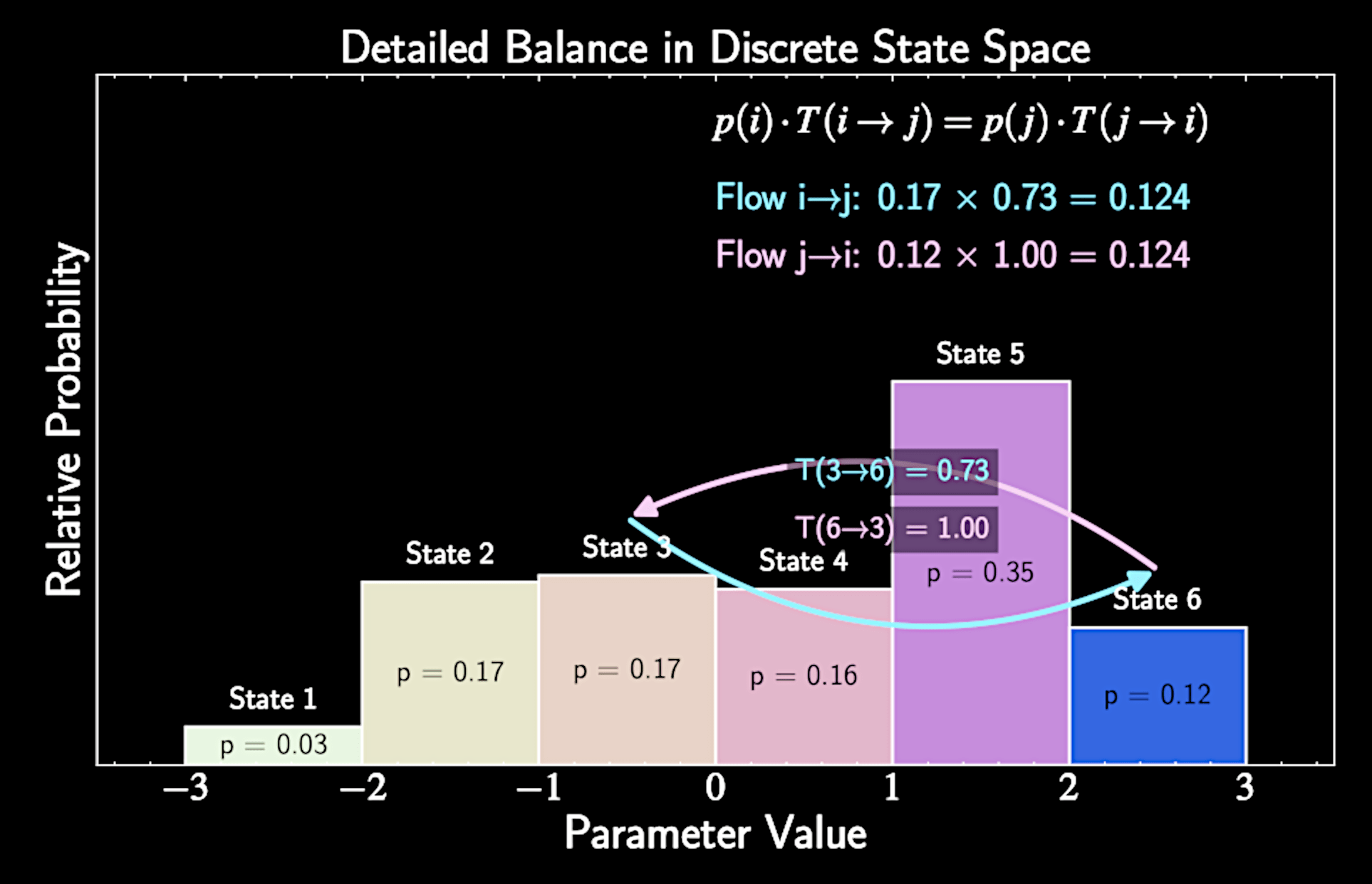
p(\mathbf{x}) T(\mathbf{x}, \mathbf{x'}) = p(\mathbf{x'}) T(\mathbf{x'}, \mathbf{x})

Proving Stationarity from Detailed Balance

p(\mathbf{x}) T(\mathbf{x}, \mathbf{x'}) = p(\mathbf{x'}) T(\mathbf{x'}, \mathbf{x})

\int p(\mathbf{x}) T(\mathbf{x}, \mathbf{x'}) d\mathbf{x} = \int p(\mathbf{x'}) T(\mathbf{x'}, \mathbf{x}) d\mathbf{x}

\int p(\mathbf{x}) T(\mathbf{x}, \mathbf{x'}) d\mathbf{x} = p(\mathbf{x'}) \int T(\mathbf{x'}, \mathbf{x}) d\mathbf{x}

\int p(\mathbf{x}) T(\mathbf{x}, \mathbf{x'}) d\mathbf{x} = p(\mathbf{x'})

Detailed Balance

When flows balance for all neighborhood pairs, population distribution remains stable

Thus, designing a transition matrix that satisfies detailed balance ensures our posterior is a stationary end point.

Constructing a Suitable Transition Matrix

We need to build a transition matrix that satisfies detailed balance

The Metropolis algorithm provides a simple, elegant solution

It decomposes transition into two steps: propose and accept/reject

Transition matrix:

T(\mathbf{x}, \mathbf{x}') = q(\mathbf{x}' | \mathbf{x}) A(\mathbf{x}, \mathbf{x}')

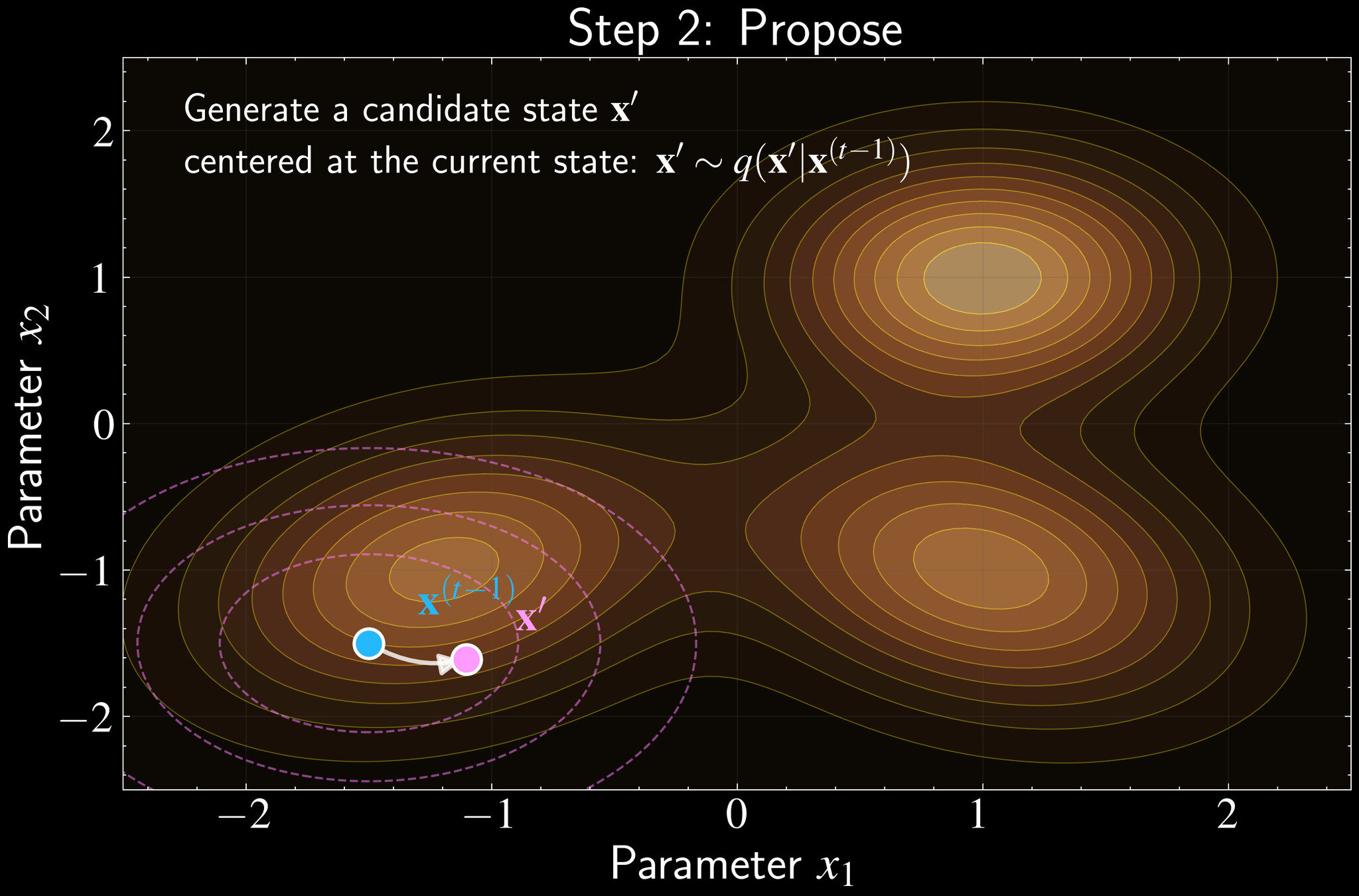
The Proposal Distribution

\(q(\mathbf{x}' | \mathbf{x})\) is the proposal distribution suggesting the next state

Metropolis uses symmetric proposals: \(q(\mathbf{x}' | \mathbf{x}) = q(\mathbf{x} | \mathbf{x}')\)

Common proposal: Gaussian centered at current position

q(\mathbf{x}' | \mathbf{x}) = \mathcal{N}(\mathbf{x}' | \mathbf{x}, \Sigma)

T(\mathbf{x}, \mathbf{x}') = q(\mathbf{x}' | \mathbf{x}) A(\mathbf{x}, \mathbf{x}')

The Acceptance Probability

Metropolis algorithm defines:

Compare posterior probability at current and proposed states

If proposed state has higher probability, always accept

A(\mathbf{x}, \mathbf{x}') = \min\left(1, \frac{p(\mathbf{x}')}{p(\mathbf{x})}\right)

T(\mathbf{x}, \mathbf{x}') = q(\mathbf{x}' | \mathbf{x}) A(\mathbf{x}, \mathbf{x}')

If lower probability, accept with probability equal to the ratio

Verifying Detailed Balance

Need to show:

Substitute transition matrix:

p(\mathbf{x}) T(\mathbf{x}, \mathbf{x}') = p(\mathbf{x}') T(\mathbf{x}', \mathbf{x})

p(\mathbf{x}) q(\mathbf{x}' | \mathbf{x}) A(\mathbf{x}, \mathbf{x}') = p(\mathbf{x}') q(\mathbf{x} | \mathbf{x}') A(\mathbf{x}', \mathbf{x})

p(\mathbf{x}) A(\mathbf{x}, \mathbf{x}') = p(\mathbf{x}') A(\mathbf{x}', \mathbf{x})

Verifying Detailed Balance (Case 1)

If \(p(\mathbf{x}') \geq p(\mathbf{x})\):

Substituting:

A(\mathbf{x}, \mathbf{x}') = 1

p(\mathbf{x}) A(\mathbf{x}, \mathbf{x}') = p(\mathbf{x}') A(\mathbf{x}', \mathbf{x})

A(\mathbf{x}, \mathbf{x}') = \min\left(1, \frac{p(\mathbf{x}')}{p(\mathbf{x})}\right)

A(\mathbf{x}', \mathbf{x}) = \frac{p(\mathbf{x})}{p(\mathbf{x}')}

p(\mathbf{x}) = p(\mathbf{x})

Verifying Detailed Balance (Case 2)

If \(p(\mathbf{x}') < p(\mathbf{x})\):

Substituting:

A(\mathbf{x}, \mathbf{x}') = \frac{p(\mathbf{x}')}{p(\mathbf{x})}

p(\mathbf{x}) A(\mathbf{x}, \mathbf{x}') = p(\mathbf{x}') A(\mathbf{x}', \mathbf{x})

A(\mathbf{x}, \mathbf{x}') = \min\left(1, \frac{p(\mathbf{x}')}{p(\mathbf{x})}\right)

A(\mathbf{x}', \mathbf{x}) = 1

p(\mathbf{x}') = p(\mathbf{x}')

Key Advantage for Astronomy

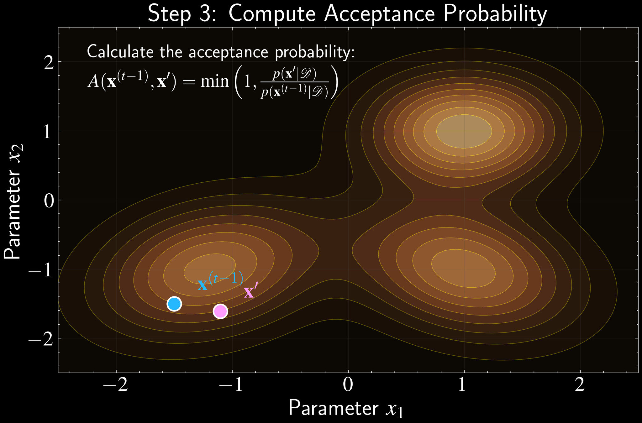
Metropolis only requires ratio of posterior probabilities:

The evidence term \(p(\mathcal{D})\) cancels out completely

Transforms an intractable sampling problem into simple likelihood and prior evaluations

\frac{p(\mathbf{x}'|\mathcal{D})}{p(\mathbf{x}|\mathcal{D})}

= \frac{p(\mathcal{D}|\mathbf{x}')p(\mathbf{x}')}{p(\mathcal{D}|\mathbf{x})p(\mathbf{x})}

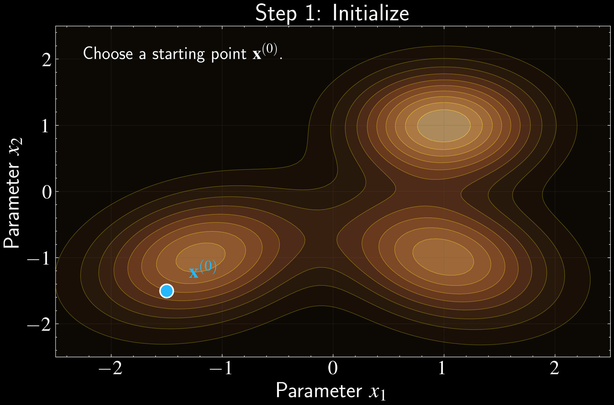
Implementation of Metropolis Algorithm

Initialize: Choose starting point \(\mathbf{x}^{(0)}\) in parameter space

Implementation of Metropolis Algorithm

For each iteration \(t = 1, 2, \ldots, T\):

Propose: Generate candidate \(\mathbf{x}' \sim q(\mathbf{x}'|\mathbf{x}^{(t-1)})\) using symmetric proposal

Initialize: Choose starting point \(\mathbf{x}^{(0)}\) in parameter space

Implementation of Metropolis Algorithm

For each iteration \(t = 1, 2, \ldots, T\):

Propose: Generate candidate \(\mathbf{x}' \sim q(\mathbf{x}'|\mathbf{x}^{(t-1)})\) using symmetric proposal

Compute acceptance probability:

Initialize: Choose starting point \(\mathbf{x}^{(0)}\) in parameter space

A(\mathbf{x}^{(t-1)}, \mathbf{x}') = \min\left(1, \frac{p(\mathbf{x}'|\mathcal{D})}{p(\mathbf{x}^{(t-1)}|\mathcal{D})}\right)

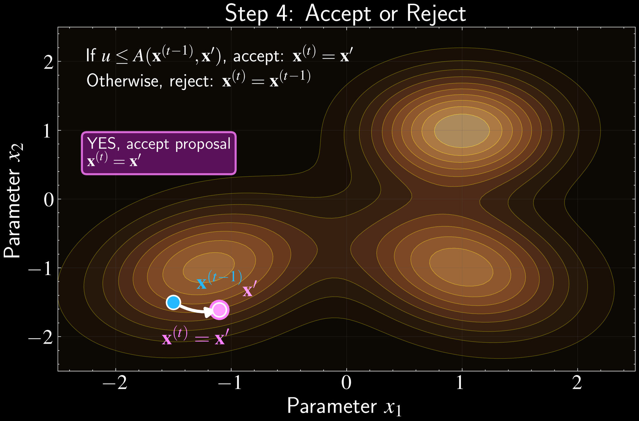
Accept/Reject:

If \(u \leq A\), accept: \(\mathbf{x}^{(t)} = \mathbf{x}'\)

Otherwise, stay put: \(\mathbf{x}^{(t)} = \mathbf{x}^{(t-1)}\)

Repeat

Draw uniform random number \(u \sim \mathcal{U}(0,1)\)

A(\mathbf{x}^{(t-1)}, \mathbf{x}') = \min\left(1, \frac{p(\mathbf{x}'|\mathcal{D})}{p(\mathbf{x}^{(t-1)}|\mathcal{D})}\right)

Convergence: no matter where we start, we eventually sample from target distribution

Uniqueness: there's only one stationary distribution our chain can converge to

Two Critical Properties: Convergence and Uniqueness

Convergence

Mathematically:

Starting distribution doesn't matter after sufficient iterations

Like tourists from anywhere in Ohio all becoming proper Columbus residents given enough time

\lim_{n\to\infty} (T^n \tilde{p})(\mathbf{x}) = p(\mathbf{x}), \quad \text{for all } \tilde{p}(\mathbf{x})

Uniqueness:

Uniqueness means if \((T p_1)(\mathbf{x}) = p_1(\mathbf{x})\) and \((T p_2)(\mathbf{x}) = p_2(\mathbf{x})\), then \(p_1(\mathbf{x}) = p_2(\mathbf{x})\)

Our travel guide must lead to only sampling from one unique distribution in the end point

Making sure our guide doesn't turn us into Cincinnati residents!

Counterexample 1: Uniqueness Failure

Neither convergence nor uniqueness is guaranteed for all Markov chains

Consider the "stay where you are" travel guide: \(T = \mathbf{Id}\)

All starting distributions are stationary: no one ever moves

Counterexample 2: Convergence Failure

Imagine Columbus with only two states: Short North and German Village

Transition matrix: \(T = \begin{bmatrix} 0 & 1 \\ 1 & 0 \end{bmatrix}\)

Travel guide: "Always move to the other neighborhood"

Has stationary distribution \(p(\mathbf{x}) = [0.5, 0.5]\) but never converges to it if we do not start with this distribution

Three Conditions for Ergodicity

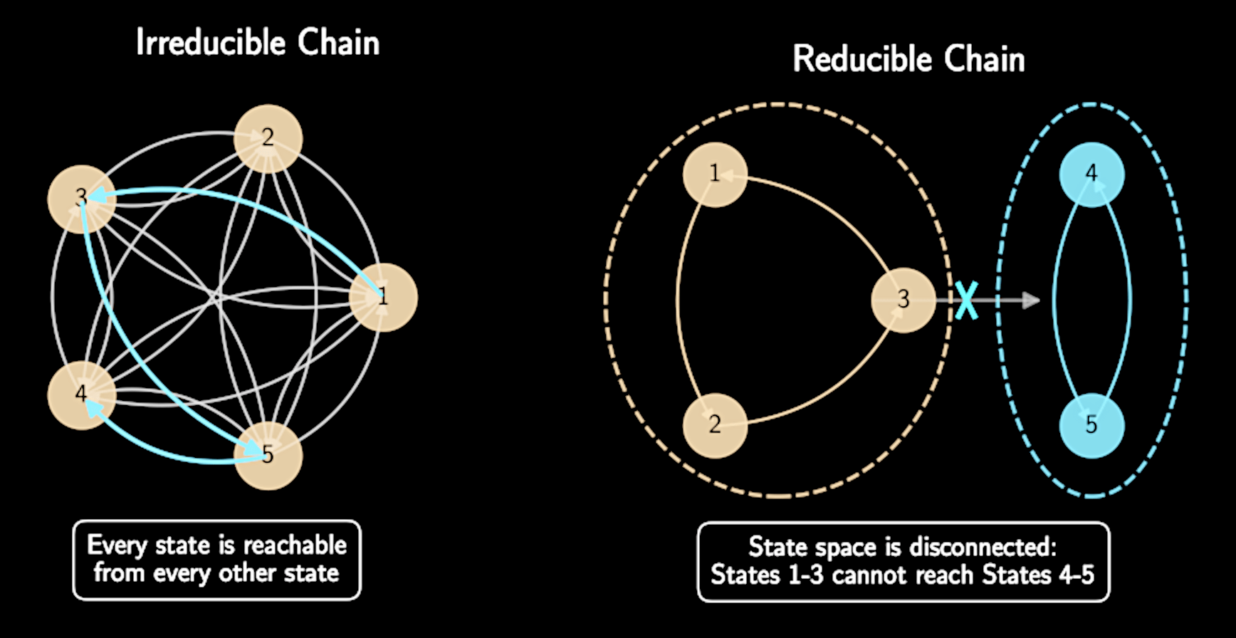
Irreducibility: Chain can go from any state to any other state in finite steps

Aperiodicity: Chain doesn't visit states in predictable cyclic patterns

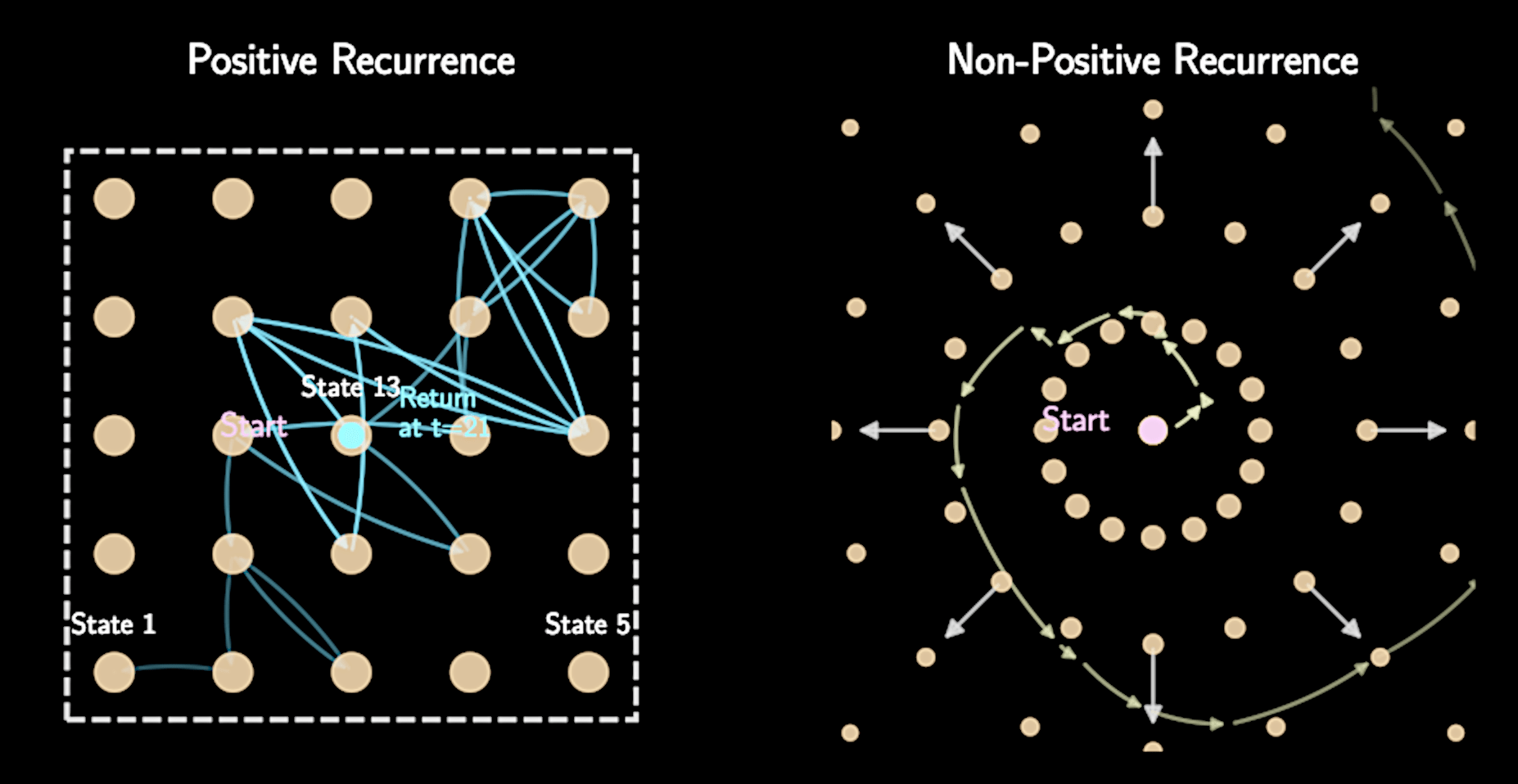
Positive recurrence: Expected time to return to any state is finite

Ergodicity guarantees both convergence and uniqueness

Irreducibility

In Columbus analogy: Ability to travel between any two neighborhoods given enough time

No isolated regions of parameter space that can't be reached

Irreducibility

In Columbus analogy: Ability to travel between any two neighborhoods given enough time

No isolated regions of parameter space that can't be reached

Can be violated if posterior has completely separated modes

Like having two separate rooms with a perfect vacuum between them

Aperiodicity and Positive Recurrence

Aperiodicity prevents oscillating behavior (recall the Short North/German Village example)

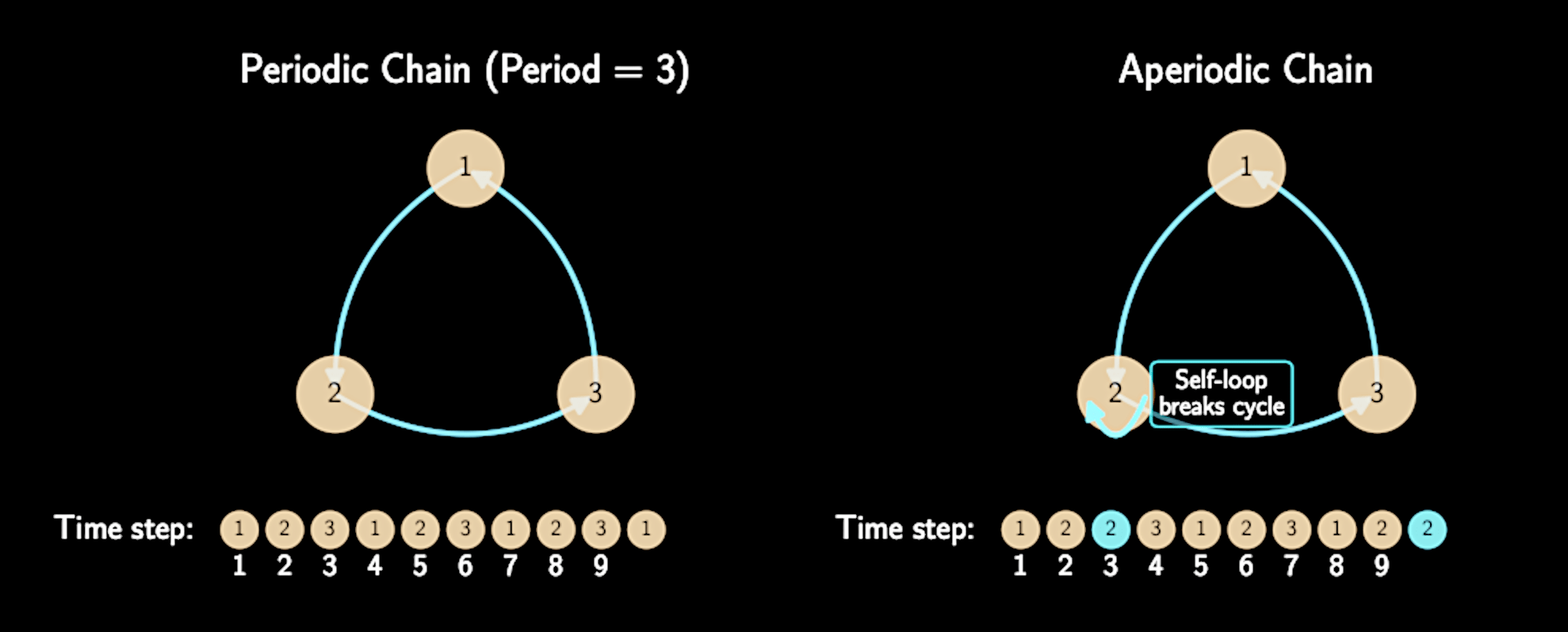
Aperiodicity and Positive Recurrence

Aperiodicity prevents oscillating behavior (recall the Short North/German Village example)

Usually satisfied by default in standard MCMC implementations

Positive recurrence prevents "wandering off to infinity"

Ensured by proper priors that bound parameter space to finite regions

Consequences of Ergodicity

When a chain is ergodic, two crucial results are guaranteed:

A unique stationary distribution exists

The chain will converge to this distribution from any starting point

Ergodicity

Ergodicity provides the theoretical foundation for why MCMC works

An ergodic chain can explore all possible states and reach equilibrium

Like gas particles exploring and equilibrating throughout a closed room

For almost all target posterior distribution, the Metropolis algorithm is naturally ergodic

Logistics

Group Project 2 - Presentation - April 16 (this Wednesday!)

Group Project 2 - Report - April 28 (no deferment)

Plan for Today :

Detailed Balance

Ergodicity

Convergence Test, Autocorrelation and Effective Sample Size

Metropolis-Hasting Algorithms and Gibbs Sampling

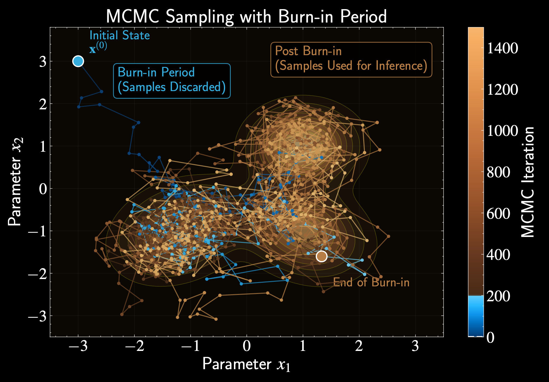
Burn-in: Warming Up the Chain

Burn-in is the warm-up period for our Markov chain

Like Columbus starting from outskirts before finding city center

Discard these initial samples when summarizing posterior

Initial samples reflect starting position, not target distribution

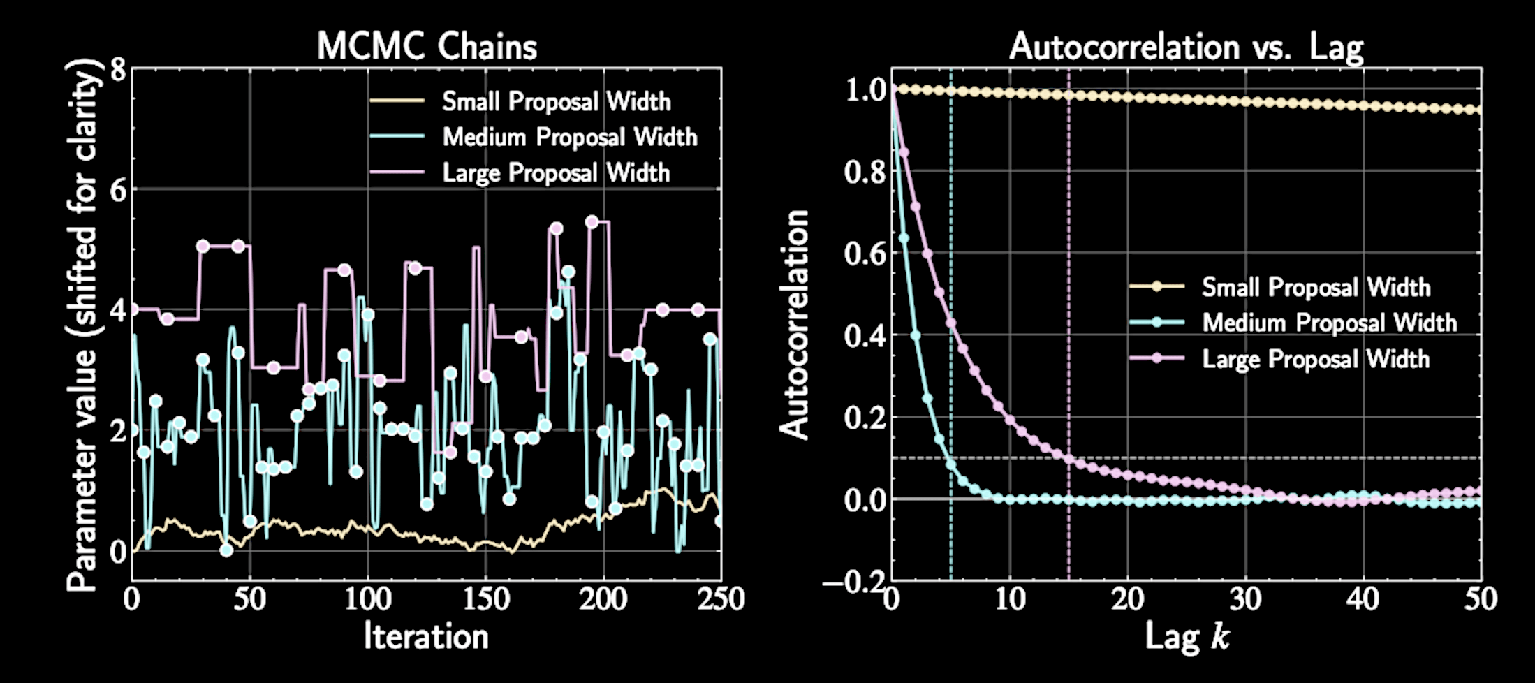
Impact of Proposal Scale in Metropolis Algorithm

Proposal choice critically affects sampling efficiency

Symmetric proposal common choice: multivariate Gaussian

q(\mathbf{x}' | \mathbf{x}) = \mathcal{N}(\mathbf{x}' | \mathbf{x}, \Sigma)

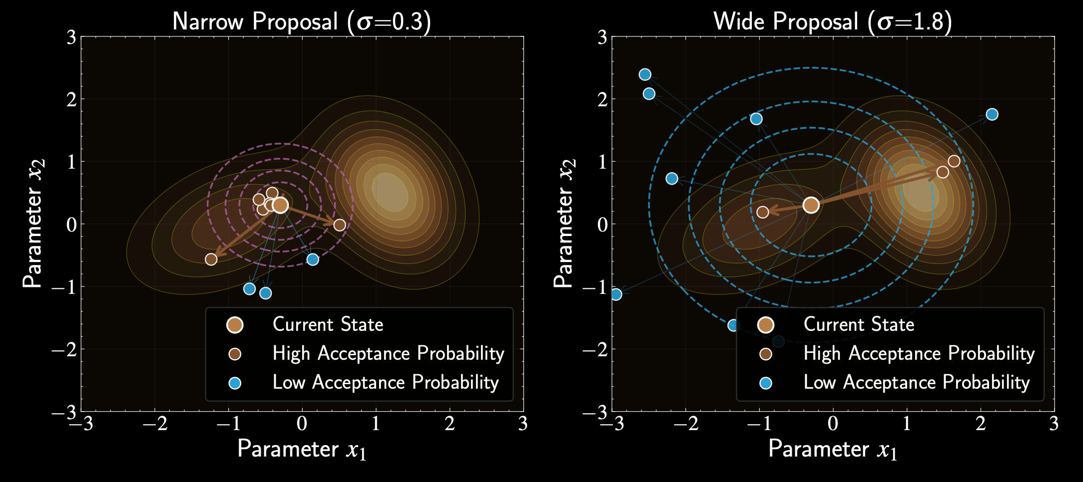
Acceptace Rate

Optimal scale: 20-40% acceptance rate for efficient exploration

Balance between moving enough and having reasonable acceptance

Too narrow proposals: high acceptance rate but slow exploration

Too wide proposals: low acceptance rate with frequent rejections

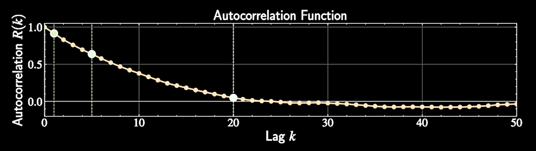
Autocorrelation: Definition and Meaning

Formal definition:

Autocorrelation at lag \( k \) measures dependency between points separated by \( k \) steps

Measures how much knowing \( X_t \) helps predict \( X_{t+k} \)

R(k) = \frac{E[(X_t - \mu)(X_{t+k} - \mu)]}{\sigma^2}

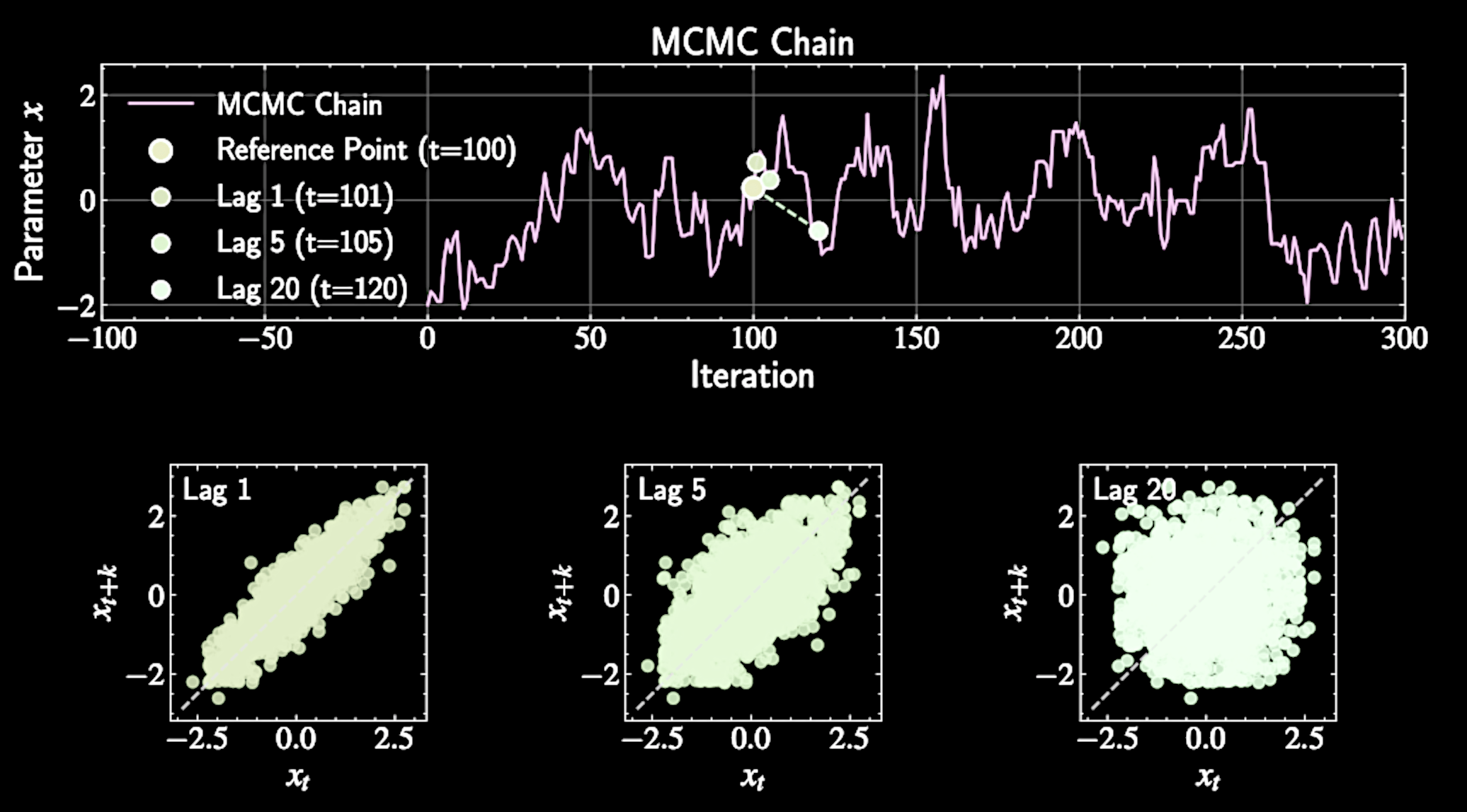
The Ergodic Perspective

Different points in same chain can be viewed as separate draws from target distribution

Well-designed MCMC chains are ergodic: irreducible, aperiodic, positive recurrent

Time averages become equivalent to ensemble averages

\hat{R}(k) = \frac{\sum_{t=1}^{N-k} (X_t - \bar{X})(X_{t+k} - \bar{X})}{\sum_{t=1}^{N} (X_t - \bar{X})^2}

Effective Sample Size (ESS)

ESS represents equivalent number of independent samples

MCMC chain of length \( N \) contains less information than \( N \) independent samples

ESS defined as:

\text{ESS} = \frac{N}{1 + 2\sum_{k=1}^{\infty}R(k)}

For independent samples: all \( R(k) = 0 \) for all \( k \), giving \( \text{ESS} = N \)

Derivation of ESS

Variance of the sample mean:

For our MCMC sample mean:

Must account for correlation between samples

\text{Var}(\bar{X}) = \frac{1}{N^2}\text{Var}\left(\sum_{i=1}^{N}X_i\right)

\bar{X} = \frac{1}{N}\sum_{i=1}^{N}X_i

\text{Var}\left(\sum_{i=1}^{N}X_i\right) = \sum_{i=1}^{N}\sum_{j = 1}^{N} \text{Cov}(X_i, X_j)

Derivation of ESS

Substituting:

In stationary chain, covariance depends only on lag:

For each lag \( k \), exactly \( (N-k) \) pairs have that lag

\text{Var}(\bar{X}) = \frac{1}{N^2}\sum_{i=1}^{N}\sum_{j=1}^{N}\sigma^2 R(|i-j|)

\text{Cov}(X_i, X_j) = \sigma^2 R(|i-j|)

\text{Var}\left(\sum_{i=1}^{N}X_i\right) = \sum_{i=1}^{N}\sum_{j = 1}^{N} \text{Cov}(X_i, X_j)

\text{Var}(\bar{X}) = \frac{\sigma^2}{N}\left[1 + 2\sum_{k=1}^{N-1}\left(1-\frac{k}{N}\right)R(k)\right]

Derivation of ESS

For independent samples, variance would be

For large \( N \), approximate as:

Equating

\frac{\sigma^2}{\text{ESS}}

\text{Var}(\bar{X}) \approx \frac{\sigma^2}{N}\left(1 + 2\sum_{k=1}^{\infty}R(k)\right)

\text{ESS} = \frac{N}{1 + 2\sum_{k=1}^{\infty}R(k)}

Denominator represents average number of correlated samples needed for one independent sample

Thinning in MCMC

Benefits: reduces storage needs, makes data more manageable, improves certain estimators

Thinning: keeping only every \( k \)-th sample to reduce correlation

Cost: discards some information since correlation between samples isn't perfect

Balance statistical precision against computational constraints

The Convergence Diagnostic

Critical challenge: determining when burn-in period is over

Including burn-in samples biases posterior estimates and leads to incorrect inferences

Target distribution is unknown - that's why we're using MCMC

Must rely on diagnostics that examine the chain's behavior

Effective Sample Size as Convergence Diagnostic

Well-converged chain: ESS grows approximately linearly with sample size after burn-in

Monitor how ESS changes as more samples are included

Low ESS relative to chain length suggests poor mixing and potential convergence issues

High ESS doesn't guarantee convergence - chain might mix well in restricted parameter space

Gelman-Rubin Method: Overview

Compare within-chain variance to between-chain variance, If chains have converged, these variances should be similar

Columbus analogy: multiple explorers should report similar neighborhood statistics

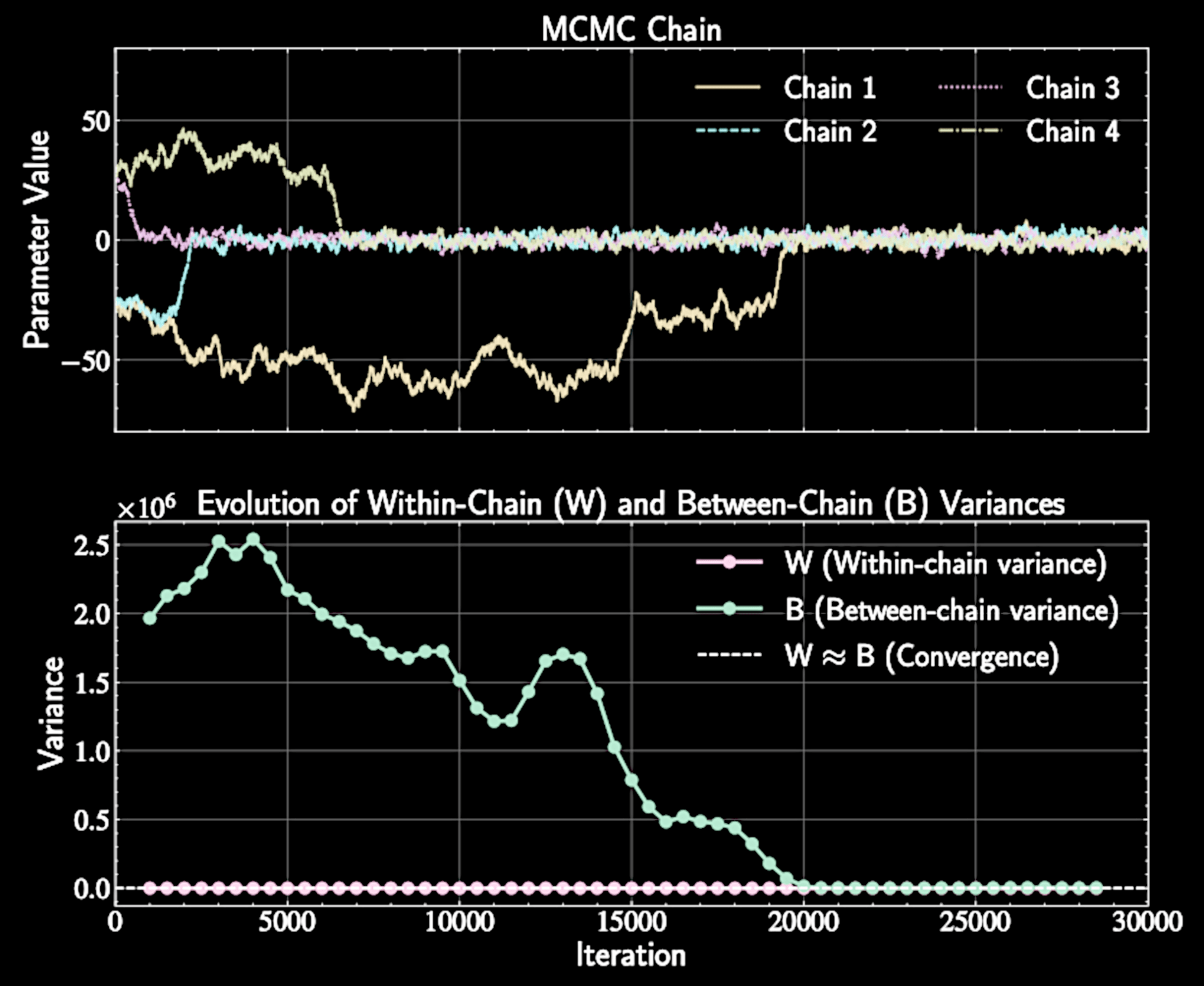
Within-Chain Variance Calculation

Within-chain variance \(W\) is the average:

For each chain \(j\), compute variance for each chain:

Represents average variance observed within individual chains

s_j^2 = \frac{1}{N}\sum_{i=1}^{N}(x_{ij} - \bar{x}_j)^2

W = \frac{1}{M}\sum_{j=1}^{M}s_j^2

Between-Chain Variance Calculation

Scale by \(n\) to make comparable to within-chain variance

Calculate variance of chain means:

When chains have converged, \(B \approx W\)

\text{Var}(\bar{x}_j) = \frac{1}{M}\sum_{j=1}^{M}(\bar{x}_j - \bar{x})^2

B = N \cdot \text{Var}(\bar{x}_j )

The Gelman-Rubin Statistic

Term \((B-W)\) represents additional variance due to incomplete convergence

Define \(\hat{R}\) statistic:

When chains have converged, \(B \approx W\) and \(\hat{R} \approx 1\)

\hat{R} = \sqrt{1 + \frac{B-W}{nW}}

Advantages and Limitations

Provides objective measure across multiple chains

Does not require knowing the true target distribution

Requires running multiple chains, increasing computational cost

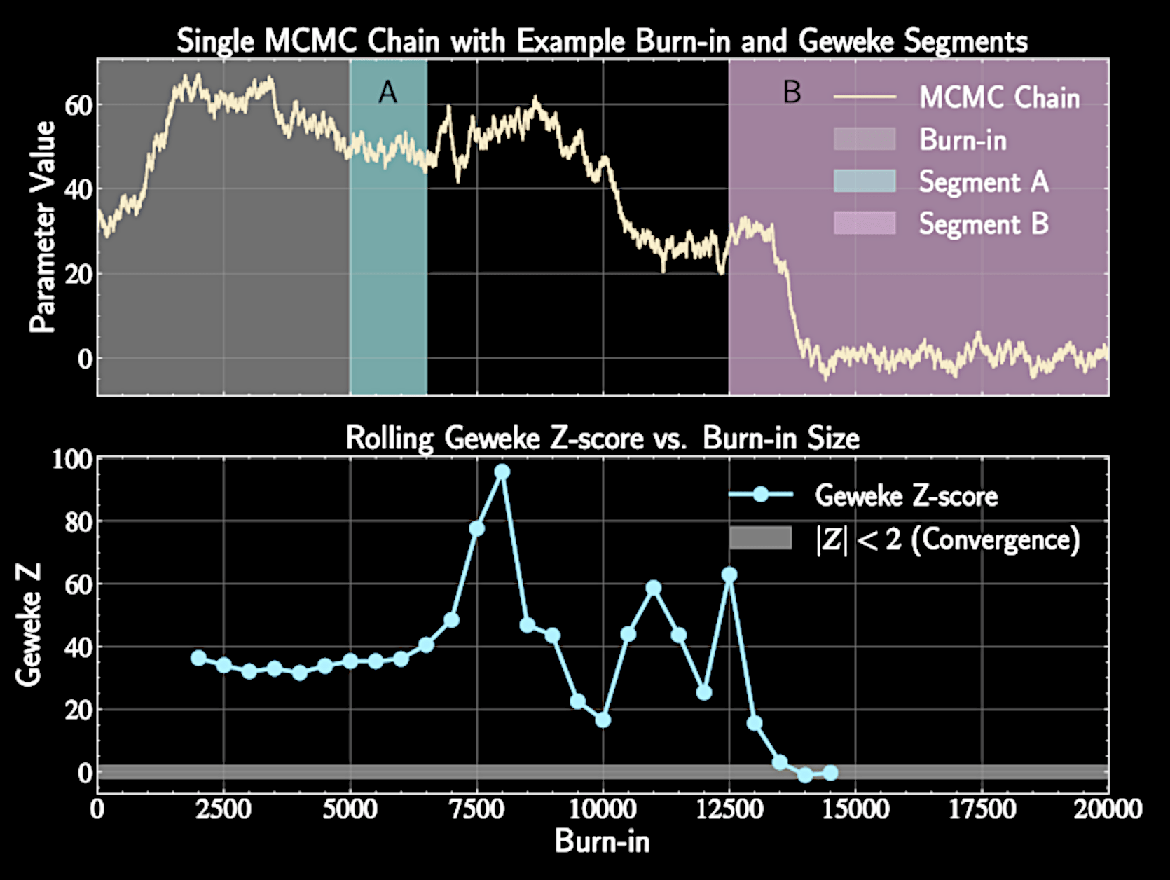
Geweke test

Run single chain and discard initial burn-in period

Assesses convergence using a single MCMC chain

Different segments of converged chain should have similar properties

Compare th first segment mean \(\bar{x}_A\) (first 10% of post-burn-in chain) with the last segment mean \(\bar{x}_B\) (typically last 50%)

Geweke test

Cannot sum infinite autocorrelation terms in practice

Samples in MCMC chain are not independent, variance of sample mean

Using windowed estimator:

\text{Var}(\bar{x}) = \frac{\sigma^2}{n}\left(1 + 2\sum_{k=1}^{\infty}R(k)\right) \equiv S

\hat{S}\equiv \frac{\hat{\sigma}^2}{N} \left(1 + 2\sum_{k=1}^{l} w(k, l) \hat{R}(k)\right), \quad w(k, l) = 1 - \frac{k}{l}

The Geweke Z-Score

Normalizes mean difference by standard error (adjusted for autocorrelation).

Compute Z-score:

Follows standard normal distribution

Z = \frac{\bar{x}_A - \bar{x}_B}{\sqrt{\hat{S}_A + \hat{S}_B}}

\( |Z| < 2 \) suggests convergence; \( |Z| > 2 \) indicates potential issues

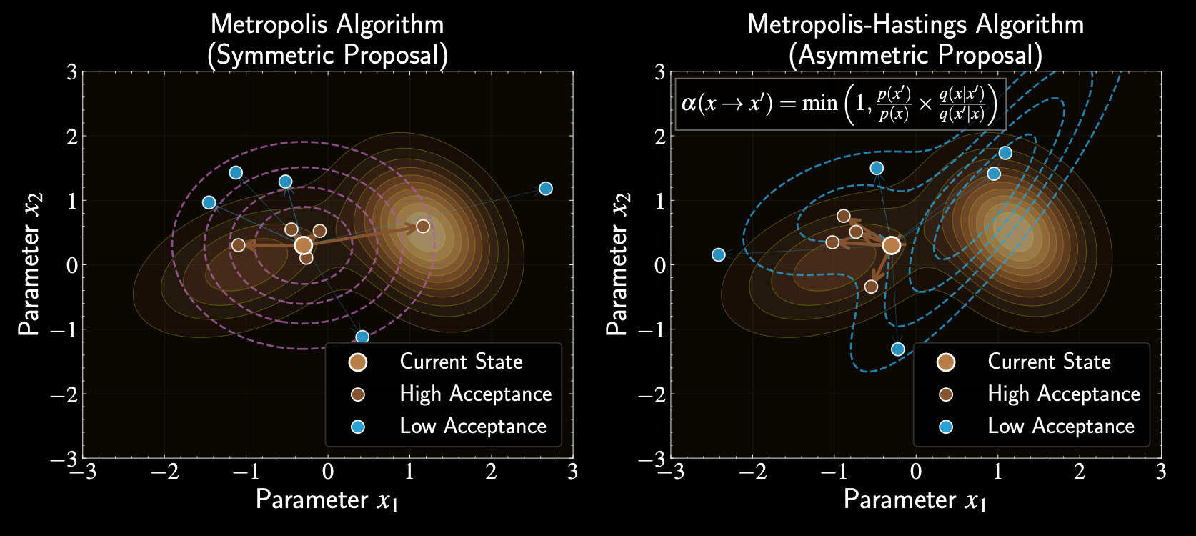
From Metropolis to Metropolis-Hastings

Metropolis-Hastings generalizes Metropolis by allowing asymmetric proposals

Standard Metropolis algorithm uses symmetric proposal distributions

Can adapt to local geometry of the posterior distribution

Leverages prior knowledge about preferred directions of movement

Transition Probability

Metropolis-Hastings acceptance probability:

Proposal distribution \(q(\mathbf{x}'|\mathbf{x})\) can be asymmetric: \(q(\mathbf{x}'|\mathbf{x}) \neq q(\mathbf{x}|\mathbf{x}')\)

Ensures detailed balance despite non-symmetric proposals, proof follows similar structure to Metropolis algorithm

A(\mathbf{x}, \mathbf{x}') = \min\left(1, \frac{p(\mathbf{x}'|\mathcal{D})q(\mathbf{x}|\mathbf{x}')}{p(\mathbf{x}|\mathcal{D})q(\mathbf{x}'|\mathbf{x})}\right)

Introduction to Gibbs Sampling

Particularly effective when joint posterior is complex but conditionals are tractable

Updates one parameter (or block of parameters) at a time

"Divide and conquer" approach to high-dimensional sampling

Efficient when conditional distributions have standard forms. Can use specialized samplers for each parameter's conditional

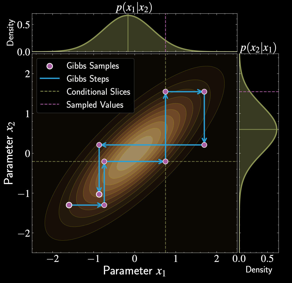
Gibbs Sampling Procedure

Sample \(x_1^{(t+1)} \sim p(x_1 | x_2^{(t)}, \ldots, x_d^{(t)})\)

Start with initial state \(\mathbf{x}^{(t)} = (x_1^{(t)}, x_2^{(t)}, \ldots, x_d^{(t)})\)

Sample \(x_2^{(t+1)} \sim p(x_2 | x_1^{(t+1)}, x_3^{(t)}, \ldots, x_d^{(t)})\)

Continue through all parameters, using updated values immediately

Gibbs as Special Case of Metropolis-Hastings

Uses conditional distribution of target as proposal

Proposal distribution for parameter:

Since Metropolis-Hastings algorithm fulfills detailed balance, so does Gibbs sampling

q_i(\mathbf{x}' | \mathbf{x}) = p(x_i' | x_1, \ldots, x_{i-1}, x_{i+1}, \ldots, x_d) \cdot \prod_{j \neq i} \delta(x_j' - x_j)

Derivation of Acceptance Probability

For Gibbs proposal:

Metropolis-Hastings acceptance:

Apply product rule, and the fact that \( x_k = x'_k \) for all \( j \neq i \)

A(\mathbf{x}, \mathbf{x}') = \min\left(1, \frac{p(\mathbf{x}')q(\mathbf{x}|\mathbf{x}')}{p(\mathbf{x})q(\mathbf{x}'|\mathbf{x})}\right)

A(\mathbf{x}, \mathbf{x}') = \min\left(1, \frac{p(\mathbf{x}') \cdot p(x_i | x_1', \ldots, x_{i-1}', x_{i+1}', \ldots, x_d')}{p(\mathbf{x}) \cdot p(x_i' | x_1, \ldots, x_{i-1}, x_{i+1}, \ldots, x_d)}\right)

p(\mathbf{x}) = p(x_i | x_1, \ldots, x_{i-1}, x_{i+1}, \ldots, x_d) \cdot p(x_1, \ldots, x_{i-1}, x_{i+1}, \ldots, x_d )

Derivation of Acceptance Probability

Always accepts proposed values (acceptance rate = 100%)

Acceptance probability simplifies to:

But acceptance probabiliy = 100% does not necessary mean effective sample size is large

A(\mathbf{x}, \mathbf{x}') = \min(1, 1) = 1

Critically depending on the correlation of the variables

Bivariate Gaussian Example

Need conditional distributions \(p(x_1 | x_2)\) and \(p(x_2 | x_1)\)

Target:

For bivariate Gaussian, conditionals are also Gaussian

\begin{pmatrix} x_1 \\ x_2 \end{pmatrix} \sim \mathcal{N}\left(\mathbf{0}, \begin{bmatrix} 1 & \rho \\ \rho & 1 \end{bmatrix}\right)

Using standard formula:

p(x_1 | x_2) = \mathcal{N}(\rho x_2, 1-\rho^2), \quad p(x_2 | x_1) = \mathcal{N}(\rho x_1, 1-\rho^2)

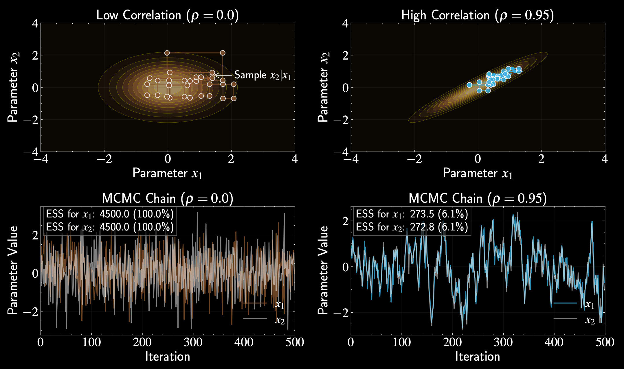
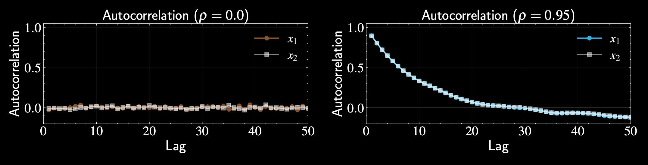
Effect of Correlation

Independent sampling in each dimension

No correlation \((\rho = 0)\):

High correlation \((\rho = 0.99)\)

p(x_1 | x_2) = p(x_2 | x_1)= \mathcal{N}(0, 1)

p(x_1 | x_2) \approx \mathcal{N}(0.99 x_2, 0.02)

p(x_1 | x_2) = \mathcal{N}(\rho x_2, 1-\rho^2)

Very small variance, new value close to previous value of other variable

Block Gibbs Sampling

Partition parameter vector into \(B\) blocks: \((\mathbf{x}_{(1)}, \mathbf{x}_{(2)}, \ldots, \mathbf{x}_{(B)})\)

Update groups of correlated parameters simultaneously

Sample \(\mathbf{x}_{(B)}^{(t+1)} \sim p(\mathbf{x}_{(B)} | \mathbf{x}_{(1)}^{(t+1)}, \ldots, \mathbf{x}_{(B-1)}^{(t+1)})\)