Graph
roychuang
Definitions
Definitions
Graph
4
5
2
3
1
數學上的圖 (Graph)
Definitions
Isomorphism
同構 (Isomorphism)
這兩張圖是一樣的 (確信)
1
3
2
4
5
1
3
2
4
5
Definitions
Vertex
點 (Vertex or Node)
3
1
2
5
4
Definitions
Edge
邊 (Edge)
1
3
2
4
5
Definitions
Path
路徑 (Path)
1
3
2
4
5
Definitions
Weight
點 or 邊權 (Weight)
比較常見的是邊權
帶權的圖叫做 Weighted-Graph
1
3
2
4
5
1
5
6
7
7
3
Definitions
Component
連通分量 / 連通塊 (Connected Component)
1
3
2
4
5
6
7
8
Definitions
Tree
聽說樹都是由上往下長的
\(N\) Nodes, \(N-1\) Edges
從一個點到另一個點永遠只有一條路
1
3
2
4
5
Definitions
Directed Graph
有向圖 (Directed Graph)
邊帶有方向
1
3
2
4
5
Definitions
Cycle
環 (Cycle)
就是字面上的意思
1
3
2
4
5
Definitions
Directed Acyclic Graph
有向無環圖 (Directed Acyclic Graph, DAG)
1
3
2
4
5
Definitions
Degree
度數 (Degree)
分為入度 (In-Degree) 和出度 (Out-Degree)
1
3
2
4
5
In: 2
Out: 1
In: 0
Out: 2
In: 2
Out: 1
In: 1
Out: 3
In: 2
Out: 0
Definitions
Simplicity
一張圖是簡單 (Simple)
代表他不含有重邊或自環
例如這張圖就不是簡單圖
1
3
2
4
5
6
重邊
自環
Representation
Representation
How To
4
5
2
3
1
Adjacency List (Prefered)
Adjacency Matrix
| 1 | 2 | 3 | 4 | 5 | |
|---|---|---|---|---|---|
| 1 | O | O | O | X | |
| 2 | O | X | O | O | |
| 3 | O | X | O | X | |
| 4 | O | O | O | O | |
| 5 | X | O | X | O |
| Node | Neighbor |
|---|---|
| 1 | 2, 3, 4 |
| 2 | 1, 4, 5 |
| 3 | 1, 4 |
| 4 | 1, 2, 3, 5 |
| 5 | 2, 4 |
Representation
Adjacency List
vector<vector<int>> al(N+1); // 1-based
al[1].push_back(3);
al[3].push_back(4);
al[4].push_back(5);
al[2].push_back(4);
al[2].push_back(5);
1
3
2
4
5
如果是無向邊就連接兩次
Representation
Weighted
vector<vector<pair<int, int>>> al(N+1);
al[1].push_back({3, 1});
al[3].push_back({4, 5});
al[4].push_back({5, 4});
al[2].push_back({4, 4});
al[2].push_back({5, 1});
1
3
2
4
5
1
1
4
4
5
Representation
Adjacency Matrix
1
3
2
4
5
1
1
4
4
5
| 1 | 2 | 3 | 4 | 5 | |
|---|---|---|---|---|---|
| 1 | 0 | 0 | 1 | 0 | 0 |
| 2 | 0 | 0 | 0 | 4 | 1 |
| 3 | 0 | 0 | 0 | 5 | 0 |
| 4 | 0 | 0 | 0 | 0 | 4 |
| 5 | 0 | 0 | 0 | 0 | 0 |
Representation
Edge List
vector<tuple<int, int, int>> el;
el.push_back({1, 3, 1});
el.push_back({3, 4, 5});
el.push_back({2, 4, 4});
el.push_back({2, 5, 1});
el.push_back({4, 5, 4});
1
3
2
4
5
1
1
4
4
5
很少用但是會用到 (?
DFS
DFS
Depth First Search
深度優先搜尋 (Depth First Search)
其中一種走訪整張圖 (暴搜) 的方法
先一路走到底 沒法走折返

DFS
Animation
3
2
4
5
1
DFS
Animation
3
5
1
4
2
DFS
Animation
3
5
1
4
2
DFS
Animation
5
1
4
2
3
DFS
Animation
1
4
2
3
5
DFS
Implementation
用遞迴實做
前面講暴搜用到的其實很多 dfs 的概念
void dfs(int parent, int current) {
	if (visited[current])
    	return;
    visited[current] = 1;
	for (const auto &nxt : adj[current]) if (nxt != parent) {
    	dfs(current, nxt);
    }
}
給你 \(N * M \) 的地圖
# 代表障礙物
. 代表你可以待的地方
算他有幾間房間
DFS
Exercise
這裡先用 dfs 做一次這題
假設我今天踩到一個空白的點
我就一路走到底 走到不能走為止
那既然都不能走了 他就是一間小房間
DFS
#include <iostream>

using namespace std;

bool can_go[1005][1005];
int N, M;

void dfs(int i, int j) {
        if (i < 0 or i >= N or j < 0 or j >= M)
                return;
        if (can_go[i][j] != true)
                return;

        can_go[i][j] = false;                  // Mark visited / Cannot go to
        dfs(i-1, j);
        dfs(i+1, j);
        dfs(i, j-1);
        dfs(i, j+1);
}

int main() {
        cin.tie(nullptr)->sync_with_stdio(false);
        cin >> N >> M;
        for (int i = 0; i < N; i++) {
                for (int j = 0; j < M; j++) {
                        char c; cin >> c;
                        if (c == '.')
                                can_go[i][j] = true;
                }
        }
        int cnt = 0;
        for (int i = 0; i < N; i++) {
                for (int j = 0; j < M; j++) {
                        if (can_go[i][j]) {      // Empty Room
                                cnt++;           // Counter + 1
                                dfs(i, j);       // How far i can reach
                        }
                }
        }
        cout << cnt << '\n';
        return 0;
}
O(N \times M)
Code
DFS
Problems
BFS
BFS
Breadth First Search
廣度優先搜尋 (Breadth First Search)
另一種走訪整張圖的方法
類似於淹水
常用於走迷宮 / 最短路

BFS
Animation
2
4
1
3
5
BFS
Animation
1
2
3
4
5
BFS
Animation
1
2
3
4
5
BFS
Animation
1
2
3
4
5
BFS
Animation
1
2
3
4
5
BFS
Implementation
queue<int> bfs;
bfs.push(1);

while (!bfs.empty()) {
	int current = bfs.front();
    bfs.pop();
    if (visited[current])
    	continue;
    visited[current] = 1;
    for (const int &nxt : adj[current]) if (!visited[nxt]) {
    	bfs.push(nxt);
    }
}
用 queue 實做
注意後面在 push 之前要把 visited 判掉
不然題目想搞你的話會被卡
給你 \(N * M \) 的地圖
# 代表障礙物
. 代表你可以待的地方
算他有幾間房間
BFS
Exercise
為什麼是同一題阿
一樣是看我可以走多遠
但我改成用 BFS 來填滿房間
BFS
#include <iostream>
#include <queue>

using namespace std;

bool can_go[1005][1005];
int N, M;

const int dx[4] = {-1, 1, 0, 0};
const int dy[4] = {0, 0, -1, 1};

void bfs(int i, int j) {
        queue<pair<int, int>> qu;
        qu.push({i, j});
        can_go[i][j] = false;           // Mark visited / Cannot go to
        while (qu.empty() == false) {
                auto [cur_i, cur_j] = qu.front();
                qu.pop();

                for (int k = 0; k < 4; k++) {
                        int new_i = cur_i + dy[k], new_j = cur_j + dx[k] ;
                        if (new_i < 0 or new_i >= N or new_j < 0 or new_j >= M)
                                continue;
                        if (can_go[new_i][new_j] == false)
                                continue;

                        can_go[new_i][new_j] = false;
                        qu.push({new_i, new_j});
                }
        }
}

int main() {
        cin.tie(nullptr)->sync_with_stdio(false);
        cin >> N >> M;
        for (int i = 0; i < N; i++) {
                for (int j = 0; j < M; j++) {
                        char c; cin >> c;
                        if (c == '.')
                                can_go[i][j] = true;
                }
        }
        int cnt = 0;
        for (int i = 0; i < N; i++) {
                for (int j = 0; j < M; j++) {
                        if (can_go[i][j]) {      // Empty Room
                                cnt++;           // Counter + 1
                                bfs(i, j);       // How far i can reach
                        }
                }
        }
        cout << cnt << '\n';
        return 0;
}
O(N \times M)
Code
BFS
Problems
Bipartite
Bipartite
Definition
二分圖 (Bipartite)
可以把所有的點都分成兩組而且不跟同組相鄰
或是可以用兩種顏色塗整張圖 而且不會有相鄰顏色相同
1
4
2
5
6
3
這張圖就不是 (讀者自證不難)
1
4
2
5
6
3
Bipartite
Exercise
Bipartite
\(N\) 位同學 \(M\) 組朋友
把全班分成兩組
組內不能有朋友
輸出一種分組方法
很顯然是 bipartite 吧
直接 DFS 下去塗色
做法:
Code
#include <iostream>
#include <vector>

using namespace std;

bool flag = 1;
vector<vector<int>> adj(1e5 + 5);
vector<int> color(1e5 + 5, 0);

void dfs(int cur, int prev) {
        color[cur] = (color[prev] == 1 ? 2 : 1);
        for (auto nxt : adj[cur]) {
                if (color[nxt] != 0) {
                        if (color[nxt] != color[cur]) {
                                continue;
                        } else {
                                flag = 0;
                                return;
                        }
                } else {
                        dfs(nxt, cur);
                }
        }
}

int main() {
        int N, M;
        cin >> N >> M;
        for (int i = 0; i < M; i++) {
                int a, b;
                cin >> a >> b;
                adj[a].push_back(b);
                adj[b].push_back(a);
        }
        color[0] = 3;
        for (int i = 1; i <= N; i++) {
                if (color[i] == 0) {
                        dfs(i, 0);
                }
        }
        if (flag) {
                for (int i = 1; i <= N; i++) cout << color[i] << " \n"[i == N];
        } else {
                cout << "IMPOSSIBLE\n";
        }
        return 0;
}
Bipartite
O(max(N, M))
Dijkstra
Dijkstra
Dijkstra's Algorithm
可以找出從一個源點 (Source) 到所有其他點的距離
複雜度是 \(O(|E|log |V|)\)

Dijkstra
Process
演算法流程 :
1. 從源點開始走
2. 往附近的點走,如果可以更新最短距離就更新
*或是已經被走過的點也不會再更新
3. 跳到目前離源點最近的點
4. 重複步驟 2~3,直到沒有人可以再更新
4
1
3
2
5
1
2
9
6
5
2
0
\(\infty\)
\(\infty\)
\(\infty\)
\(\infty\)
Dijkstra
Process
4
3
2
5
1
2
9
6
5
2
0
\(\infty\)
\(\infty\)
\(\infty\)
\(\infty\)
1
演算法流程 :
1. 從源點開始走
2. 往附近的點走,如果可以更新最短距離就更新
*或是已經被走過的點也不會再更新
3. 跳到目前離源點最近的點
4. 重複步驟 2~3,直到沒有人可以再更新
Dijkstra
Process
4
3
2
5
1
2
9
6
5
2
0
5
\(\infty\)
9
1
1
演算法流程 :
1. 從源點開始走
2. 往附近的點走,如果可以更新最短距離就更新
*或是已經被走過的點也不會再更新
3. 跳到目前離源點最近的點
4. 重複步驟 2~3,直到沒有人可以再更新
Dijkstra
Process
4
3
2
5
1
2
9
6
5
2
0
5
\(\infty\)
9
1
1
演算法流程 :
1. 從源點開始走
2. 往附近的點走,如果可以更新最短距離就更新
*或是已經被走過的點也不會再更新
3. 跳到目前離源點最近的點
4. 重複步驟 2~3,直到沒有人可以再更新
Dijkstra
Process
4
3
2
5
1
2
9
6
5
2
0
5
\(\infty\)
3
1
1
演算法流程 :
1. 從源點開始走
2. 往附近的點走,如果可以更新最短距離就更新
*或是已經被走過的點也不會再更新
3. 跳到目前離源點最近的點
4. 重複步驟 2~3,直到沒有人可以再更新
Dijkstra
Process
3
2
5
1
2
9
6
5
2
0
5
\(\infty\)
3
1
1
4
演算法流程 :
1. 從源點開始走
2. 往附近的點走,如果可以更新最短距離就更新
*或是已經被走過的點也不會再更新
3. 跳到目前離源點最近的點
4. 重複步驟 2~3,直到沒有人可以再更新
Dijkstra
Process
3
2
5
1
2
9
6
5
2
0
5
8
3
1
1
4
演算法流程 :
1. 從源點開始走
2. 往附近的點走,如果可以更新最短距離就更新
*或是已經被走過的點也不會再更新
3. 跳到目前離源點最近的點
4. 重複步驟 2~3,直到沒有人可以再更新
Dijkstra
Process
3
2
5
1
2
9
6
5
2
0
5
8
3
1
1
4
演算法流程 :
1. 從源點開始走
2. 往附近的點走,如果可以更新最短距離就更新
*或是已經被走過的點也不會再更新
3. 跳到目前離源點最近的點
4. 重複步驟 2~3,直到沒有人可以再更新
Dijkstra
Process
3
2
5
1
2
9
6
5
2
0
5
7
3
1
1
4
演算法流程 :
1. 從源點開始走
2. 往附近的點走,如果可以更新最短距離就更新
*或是已經被走過的點也不會再更新
3. 跳到目前離源點最近的點
4. 重複步驟 2~3,直到沒有人可以再更新
Dijkstra
Process
3
2
5
1
2
9
6
5
2
0
5
7
3
1
1
4
演算法流程 :
1. 從源點開始走
2. 往附近的點走,如果可以更新最短距離就更新
*或是已經被走過的點也不會再更新
3. 跳到目前離源點最近的點
4. 重複步驟 2~3,直到沒有人可以再更新
Dijkstra
Implementation
using lli = long long int;
const lli INF = 1e18;

vector<lli> dijkstra(vector<vector<pair<int, lli>>> &adj, int N, int from) {
    vector<lli> dist(N+1, INF);      // 1 based
    vector<bool> visited(N+1, 0);
    dist[from] = 0;
    priority_queue<pair<lli, int>, vector<pair<lli, int>>, greater<pair<lli, int>>> pq;
    pq.push({0, from});

    while (!pq.empty()) {
        auto [_, cur] = pq.top();
        pq.pop();
        if (visited[cur]) continue;
        visited[cur] = 1;

        for (auto &[nxt, weight] : adj[cur]) {
            if (dist[nxt] > dist[cur] + weight) {
                dist[nxt] = dist[cur] + weight;
                pq.push({dist[nxt], nxt});
            }
        }
    }

    return dist;
}
以 priority_queue 作為 min heap
Problems
Dijkstra
Bellman-Ford
Bellman-Ford
Bellman-Ford Algorithm
可以找出從一個源點 (Source) 到所有其他點的距離
複雜度是 \(O(|E|\cdot|V|)\)
Process
演算法流程 :
1. 跑遍每條邊,如果可以減少距離就更新
2. 重複 \(N-1\) 次,或重複直到無法再減少距離 (減少距離又稱為 Relax, 鬆弛)
4
3
2
5
1
2
9
6
5
2
0
\(\infty\)
\(\infty\)
\(\infty\)
\(\infty\)
Bellman-Ford
1
Process
演算法流程 :
1. 跑遍每條邊,如果可以減少距離就更新
2. 重複 \(N-1\) 次,或重複直到無法再減少距離 (減少距離又稱為 Relax, 鬆弛)
4
3
2
5
1
2
9
6
5
2
0
5
\(\infty\)
9
1
Bellman-Ford
1
Process
演算法流程 :
1. 跑遍每條邊,如果可以減少距離就更新
2. 重複 \(N-1\) 次,或重複直到無法再減少距離 (減少距離又稱為 Relax, 鬆弛)
4
3
2
5
1
2
9
6
5
2
0
5
7
3
1
Bellman-Ford
1
Process
演算法流程 :
1. 跑遍每條邊,如果可以減少距離就更新
2. 重複 \(N-1\) 次,或重複直到無法再減少距離 (減少距離又稱為 Relax, 鬆弛)
4
3
2
5
1
2
9
6
5
2
0
5
7
3
1
Bellman-Ford
1
Negative Cycle
跑到第 \(N\) 次還可以 Relax 就代表有
Negative Cycle
4
3
2
5
-1
-1
-1
6
5
2
Bellman-Ford
1
Implementation
Bellman-Ford
using lli = long long int;
const lli INF = 1e18;

bool relaxed, neg_cycle = 0;
vector<lli> distance(N+1, INF);
vector<bool> connected_to_N(N+1, 0), reachable(N+1, 0);
distance[1] = 0, connected_to_N[N] = 1, reachable[1] = 1;

for (int i = 1; i <= N - 1; i++) {
	relaxed = 0;
	for (const auto &[u, v, w] : edge_list) {
    	if (distance[v] > distance [u] + w) {
        	distance[v] = distance[u] + w;
            relaxed = 1;
        }

        if (reachable[u]) reachable[v] = 1;
        if (connected_to_N[v]) connected_to_N[u] = 1;

        if (!relaxed)
        	break;
    }
}

for (const auto &[u, v, w] : edge_list) {
	iuf (reachable[u] and distance[v] > distance[u] + w and connected_to_N[v]) {
    	cout << "Negative Cycle Found !" << endl;
        neg_cycle = 1;
        break;
    }
}
bellman-ford 會需要把圖存成 edge_list
如果沒有更新長度 (Relax) 就停止
Exercise
\(N\) (\(1 \leq N \leq 2500\)) 間海關小房間
\(M\) (\(1 \leq M \leq 5000\)) 條單向隧道
每個隧道有分數 \(x\) (有正有負)
求從 \(1\) 走到 \(N\) 最大總分
如果會變成無限大輸出 \(-1\)
注意到這題是 Bellman-Ford 的變體
Bellman-Ford
變成我的目標是求最長路 如果會有正環輸出 -1
Floyd–Warshall
Floyd-Warshall
Floyd–Warshall Algorithm
可以找出從所有點到所有點的距離
複雜度是 \(O(|V|^3)\)

Process
演算法流程 :(太抽象了,有動畫也看不懂,我就不做動畫了)
用 adjacency matrix 存圖
跑遍每個中間點 k,對於每兩個點 i, j
如果 distance( \(i \rightarrow k \rightarrow j\) ) < distance( \(i \rightarrow j\) ) 就更新
4
3
2
5
1
2
9
7
5
2
1
Floyd-Warshall
| 1 | 2 | 3 | 4 | 5 | |
|---|---|---|---|---|---|
| 1 | 0 | 5 | 9 | 1 | |
| 2 | 5 | 0 | 2 | ||
| 3 | 2 | 0 | 7 | ||
| 4 | 9 | 7 | 0 | 2 | |
| 5 | 1 | 2 | 0 |
\(\infty\)
\(\infty\)
\(\infty\)
\(\infty\)
\(\infty\)
\(\infty\)
\(\infty\)
\(\infty\)
Process
4
3
2
5
1
2
9
7
5
2
1
Floyd-Warshall
| 1 | 2 | 3 | 4 | 5 | |
|---|---|---|---|---|---|
| 1 | 0 | 5 | 1 | ||
| 2 | 5 | 0 | 2 | ||
| 3 | 2 | 0 | 7 | ||
| 4 | 7 | 0 | 2 | ||
| 5 | 1 | 2 | 0 |
7
3
7
3
8
6
8
6
8
8
演算法流程 :(太抽象了,有動畫也看不懂,我就不做動畫了)
用 adjacency matrix 存圖
跑遍每個中間點 k,對於每兩個點 i, j
如果 distance( \(i \rightarrow k \rightarrow j\) ) < distance( \(i \rightarrow j\) ) 就更新
Implementation
Floyd-Warshall
for (int k = 1; k <= N; k++) {
    for (int i = 1; i <= N; i++) {
        for (int j = 1; j <= N; j++) {
            adj_matrix[i][j] = min(
            	adj_matrix[i][k] + adj_matrix[k][j],
                adj_matrix[i][j]
			);
        }
    }
}
好懂多了
記得順序 k, i, j
Exercise
\(N\) (\(1 \leq N \leq 500\)) 個點
\(M\) (\(1 \leq M \leq N^2\)) 條雙向邊
\(Q\) (\(1 \leq Q \leq 10^5\)) 筆詢問
求兩點最短距離
\( N \leq 500, Q \leq 10^5\)
Floyd-Warshall
計算 \( O(N^3) \), 查詢 \(O(1)\)
A*
A*
A* Algorithm
Dijkstra 還是太慢 ?
BFS 複雜度太爛 ?
A*
How it works
一樣用 min heap
Dijkstra 原本是根據源點到點的距離
作為比較標準放進 min heap
A* 的想法是我先拿一個唬爛函數 h(x)
他可以大致上評估這個點到終點的距離
(而且評估結果要小於真實距離)
以 distance(x) + h(x) 作為比較標準放進 min heap
而最常見的 h(x) 就是拿曼哈頓距離 (Manhattan Distance)
A*
Example
\( N \times M (1 \leq N, M \leq 1000) \) 的迷宮
找從入口 A 到出口 B 的最短路徑
輸出 YES, 路徑長, 走法
沒有輸出 NO
先用 A* 做這題
我跟 Dijkstra 一樣使用 min heap
並且拿曼哈頓距離 (\(|x_2 - x_1| + |y_2 - y_1|\)) 作為
唬爛 (啟發式 , Heuristic) 函數 h(x)
每次走到 distance(x, y) + h(x, y) 最小的點
Tree
Tree
Definitions
聽說樹都是由上往下長的
\(N\) Vertices, \(N-1\) Edges
從任何點到另外一點只有一條路
1
3
2
4
5

Tree
Definitions
最上面叫做樹根 (root)
相對上面稱為父節點 (parent)
相對下面的稱為子節點 (child)
沒有子節點的稱為葉節點 (leaf)
1
3
2
4
5
Leaf
Root
Root
Parent
Child
Tree
今天還不會細講樹
DSU
DSU
Union-Find Structure
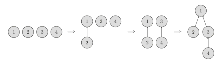
DSU
How it works
我們把 N 個點蓋一個森林
合併:把兩棵樹連成一棵
查詢:找跟節點是誰
1
3
2
4
5
Root = 1
Root = 1
Root = 2
Root = 2
Root = 2
DSU
How it works
我們把 N 個點蓋一個森林
合併:把兩棵樹連成一棵
查詢:找跟節點是誰
1
3
2
4
5
Root = 1
Root = 1
Root = 1
Root = 1
Root = 1
DSU
Naive Implementation
int find_set(int v) {
    if (v == parent[v])
        return v;
    return find_set(parent[v]);
}

void union_sets(int a, int b) {
    a = find_set(a);
    b = find_set(b);
    if (a != b)
        parent[b] = a;
}
DSU
Union by size
void union_sets(int a, int b) {
    a = find_set(a);
    b = find_set(b);
    if (a != b) {
        if (size[a] < size[b])
            swap(a, b);
        parent[b] = a;
        size[a] += size[b];
    }
}
可以減小 find_set 花的時間
DSU
Path Compression
struct DSU {
    int root[100005];

    void init(int n) {
        for (int i = 1; i <= n; i++) root[i] = i;
    }

    void unite(int a, int b) {
        // find roots
        a = find_root(a);
        b = find_root(b);
        root[b] = a; // merge root
    }

    int find_root(int x) {
        if (root[x] == x) return x;
        root[x] = find_root(root[x]); // pre save the roots
        return root[x];
    }

} dsu;
O(\alpha(N))
DSU
補充一點怪東西
Spanning Tree
Spanning Tree
Minimum Spanning Tree
最小生成樹 (Minimum Spanning Tree)
用最小的總成本把所有點連起來的方法
如右圖就是左圖的其中一種最小生成樹 (可能有多種)
1
2
5
3
6
4
3
6
5
5
2
3
9
7
1
2
5
3
6
4
3
5
2
3
7
Spanning Tree
Kruskal’s algorithm
先存 edge list
根據邊權大小把邊做排序
如果邊上兩點 A B 已經連通就跳過
否則把 A B 連起來
Spanning Tree
Kruskal’s algorithm
sort(edges.begin(), edges.end(), [](auto &e1, auto &e2) {
	return (get<2>(e1)) < (get<2>(e2));
});

for (const auto &[a, b] : edge_list) {
	if (dsu.find_root(a) == dsu.find_root(b))
    	continue;

    dsu.unite(a, b);
    adj[a].push_back(b);
    adj[b].push_back(a);
}
O(|E|\log |E| + |V|\alpha(|V|))
Spanning Tree
Prim’s algorithm
從某個點開始
找 "目前邊權最小" 的邊連過去
一樣能連 A B 就連起來
類似 Dijkstra
Spanning Tree
Prim’s algorithm
priority_queue<tuple<lli, int, int>> pq;
pq.push({0, 1, 0});

while (!pq.empty()) {
        const auto [w, cur, parent] = pq.top();
        pq.pop();
        if (visited[cur])
                continue;
        visited[cur] = 1;

        if (dsu->same_component(cur, parent))
                continue;

        dsu->unite(cur, parent);

        adj_spanning_tree[parent].push_back(cur, -w);
        adj_spanning_tree[cur].push_back(parent, -w);

        cost -= w;
        components--;

        for (const auto &[nxt, nw] : adj[cur]) if (!visited[nxt]) {
                pq.push({-nw, nxt, cur});
        }
}
O(|E|\log|V| + |V|\alpha(|V|))
Spanning Tree
Example
Thanks

Graph
By Roy Chuang


