Machine Learning
roychuang
Winter Camp Ver.
Background
Background
人工智慧 (artificial intelligence, AI) ,由愛倫·圖靈 (Alan Turing) 所提出的概念,代表使用電腦去模擬人類具有智慧的行為,例如語言、學習、思考、論證、創造等等。
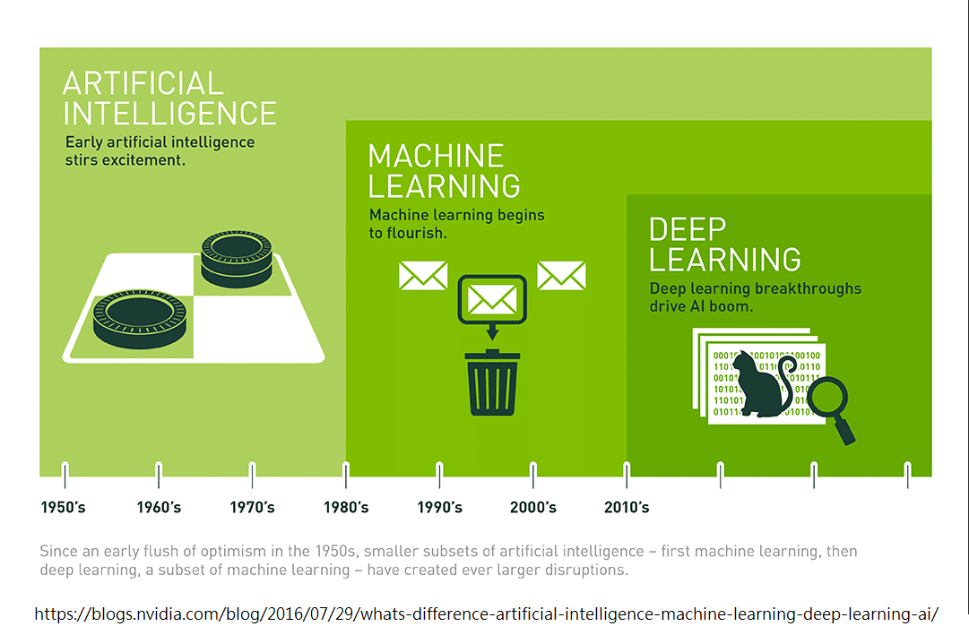
機器學習 (Machine Learning, ML),1959 年被 IBM 員工 Arthur Samuel 提出,代表透過統計學,讓機器自己做學習,而並非用一條指令一個動作的方式,來製造人工智慧。
Background
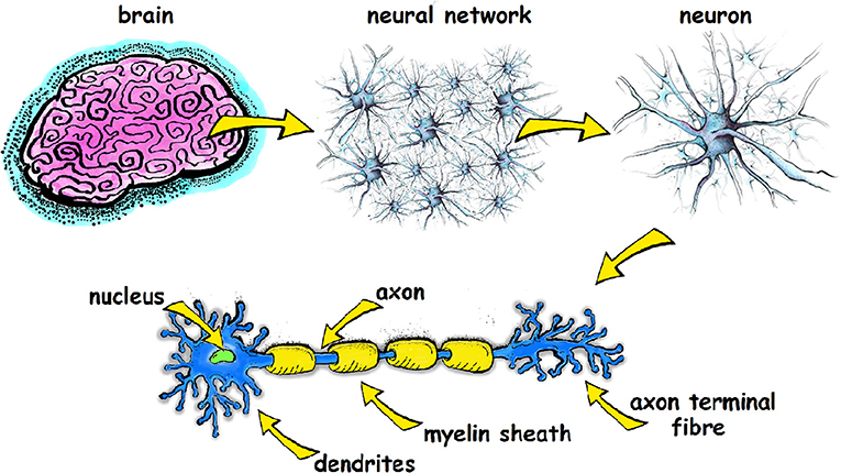
深度學習 (Deep Learning),一種機器學習的方法,我們模擬人類大腦神經元的運作模式,由許多神經細胞構成神經網路,經歴學習的過程,藉此訓練一個 AI。
深度學習又可以分為 Multilayer perceptron (MLP), Recurrent neural network (RNN), convolutional neural network (CNN) 等等。
Background
Neural Network
Neural Network
Human Brain
Neural Network
\(x_1\)
\(x_2\)
\(x_3\)
\(y_1\)
\(y_2\)
Input Layer
Hidden Layers
Output
Layer
Neural Network (NN)
Neuron
\(W_1\)
\(W_2\)
b
\(x_1\)
\(x_2\)
\(z\)
\(z = x_1w_1 + x_2w_2 + b\)
Neural Network
Neuron
Neuron
\(W_1\)
\(W_2\)
b
\(x_1\)
\(x_2\)
\(z\)
Activation Function

Neural Network
Example
1
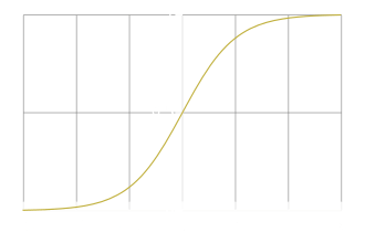
Activation : Sigmoid \(\sigma(z) = \frac{1}{1+e^{-z}} \)
-1
1
0
0
0
-2
2
1
-2
-1
1
2
-1
-2
1
3
-1
-1
4
4
0.98
-2
0.12
0.86
0.11
0.62
0.83
Neural Network
Training
Training
Process
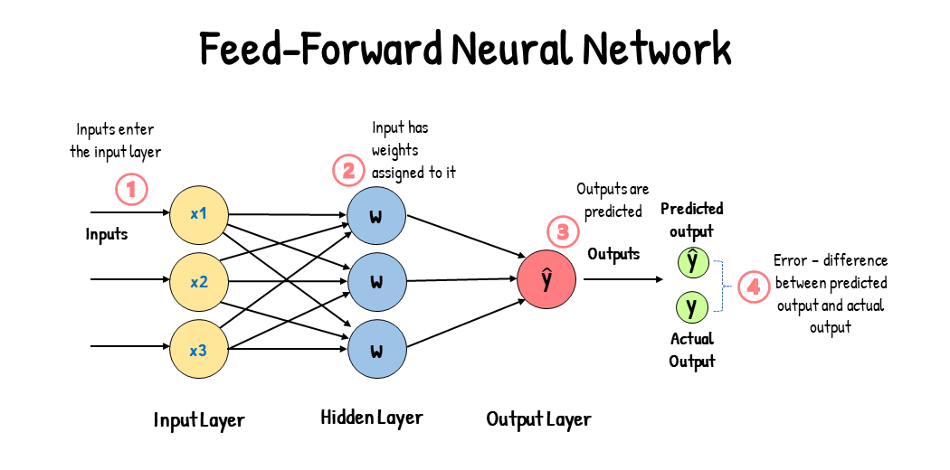
- 目標:給定輸入之後,可以得到期望的輸出。
- 先隨機給定一些權重 \(\vec{W}\) 和輸入 \(\vec{X }\),接著透過誤差函數 (Loss Function) 比較輸出 \(\hat{y}\) 和正解 \(y\) 的差距 (Loss),最後根據 Loss 去調整各個 Weight 和 Bias。
Training
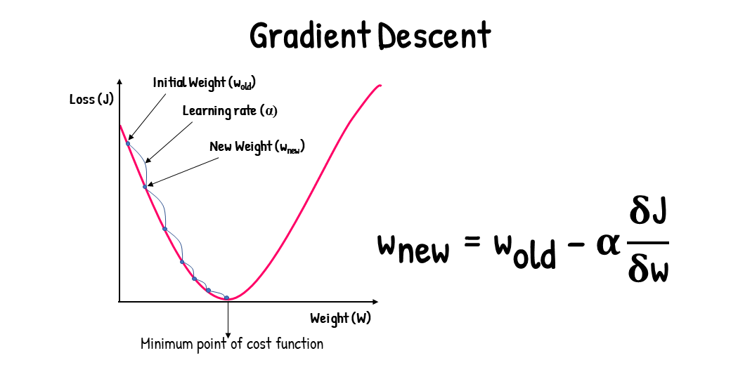
Gradient Descent
-
調整 Weight 和 Bias 的過程稱為最佳化 (Optimization, 最常用的方法是梯度下降 Gradient Descent)。
-
Gradient Descent 指的是,把誤差畫成函數圖形以後,根據斜坡的方向,朝著更低的那個點走,以此來更新 Weights
Training
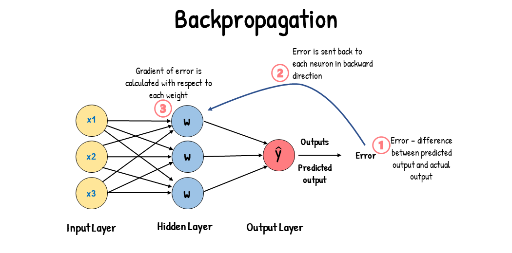
Backpropagation
- 加速 optimization
- 得到其中一個 Weight 的 Gradient 以後透過一層層回推的方式快速反推所有其他 Weight 的 Gradient
MNIST & Keras
MNIST & Keras
MNIST
- Modified National Institute of Standards and Technology database
- 手寫數字資料集
- 裡面包含的是 70000 組 (60000組訓練資料 + 10000組考試資料) 圖片 (黑底白字的手寫數字) 和對應的數字

MNIST & Keras
Keras
- 一個開源的神經網路前端
- 後端通常使用 tensorflow
- 用類似拼積木的方式來建構神經網路
MNIST & Keras
Installation
For Linux User : 要先處理 Nvidia Driver 💀
安裝相關模組 :
推薦 conda (miniforge) 管理器 (可以避免許多 python 特有的怪版本問題)
conda install cudatoolkit cudnn python tensorflow-gpu keras numpy pandas matplotlib pillow scikit-learn jupyterlab如果沒有 Nvidia GPU,那就不用安裝 cuda 和 cudnn,tensorflow 改為 tensorflow-cpu

Math Warning
Matrices
Matrix
Matrices
\left[
\begin{array}{cccc}
x_{00} & x_{10} & \cdots & x_{m0} \\
x_{01} & x_{11} & \cdots & x_{m1} \\
\vdots & \vdots & \ddots & \vdots \\
x_{0n} & x_{1n} & \cdots & x_{mn}
\end{array}
\right]
- 算是一種資料結構
- 用來把一堆數字包起來/一起做運算
Add
\left[
\begin{array}{cc}
1 & 2 \\
3 & 4 \\
\end{array}
\right]
+ 5 =
\left[
\begin{array}{cc}
6 & 7 \\
8 & 9 \\
\end{array}
\right]
\left[
\begin{array}{cc}
1 & 2 \\
3 & 4 \\
\end{array}
\right]
+
\left[
\begin{array}{cc}
4 & 3 \\
2 & 1 \\
\end{array}
\right]
=
\left[
\begin{array}{cc}
5 & 5 \\
5 & 5
\end{array}
\right]
Matrices
矩陣加矩陣的話大小要一樣
Multiply a Scalar
5 \cdot
\left[
\begin{array}{cc}
1 & 2 \\
3 & 4 \\
\end{array}
\right]
=
\left[
\begin{array}{cc}
5 & 10 \\
15 & 20 \\
\end{array}
\right]
Matrices
Vector & dot product
\vec{A} =
\left[
\begin{array}{c}
1 \\
1 \\
4 \\
\end{array}
\right]
Matrices
\vec{B} =
\left[
\begin{array}{c}
5 \\
1 \\
4 \\
\end{array}
\right]
\vec{A} \cdot \vec{B} =
(
1 \cdot 5 +
1 \cdot 1 +
4 \cdot 4
)
= 22
Transpose
A =
\left[
\begin{array}{cc}
1 & 2 \\
3 & 4 \\
5 & 6 \\
\end{array}
\right]
Matrices
A^T =
\left[
\begin{array}{ccc}
1 & 3 & 5 \\
2 & 4 & 6 \\
\end{array}
\right]
Multiplication
\left[
\begin{array}{ccc}
1 & 2 & 3 \\
4 & 5 & 6 \\
\end{array}
\right]
\cdot
\left[
\begin{array}{c}
1 & 5 \\
1 & 1 \\
4 & 4 \\
\end{array}
\right]
=
\left[
\begin{array}{cc}
17 & 19 \\
33 & 49 \\
\end{array}
\right]
Matrices
\left[
\begin{array}{c}
1 & 5 \\
1 & 1 \\
4 & 4 \\
\end{array}
\right]
\left[
\begin{array}{ccc}
1 & 2 & 3 \\
4 & 5 & 6 \\
\end{array}
\right]
\left[
\begin{array}{cc}
15 & 19 \\
33 & 49 \\
\end{array}
\right]
1 \cdot 1 + 2 \cdot 1 + 3 \cdot 4 = 15
Multiplication
Matrices
\left[
\begin{array}{c}
1 & 5 \\
1 & 1 \\
4 & 4 \\
\end{array}
\right]
\left[
\begin{array}{ccc}
1 & 2 & 3 \\
4 & 5 & 6 \\
\end{array}
\right]
\left[
\begin{array}{cc}
15 & 19 \\
33 & 49 \\
\end{array}
\right]
1 \cdot 5 + 2 \cdot 1 + 3 \cdot 4 = 19
\left[
\begin{array}{ccc}
1 & 2 & 3 \\
4 & 5 & 6 \\
\end{array}
\right]
\cdot
\left[
\begin{array}{c}
1 & 5 \\
1 & 1 \\
4 & 4 \\
\end{array}
\right]
=
\left[
\begin{array}{cc}
17 & 19 \\
33 & 49 \\
\end{array}
\right]
Multiplication
Matrices
\left[
\begin{array}{c}
1 & 5 \\
1 & 1 \\
4 & 4 \\
\end{array}
\right]
\left[
\begin{array}{ccc}
1 & 2 & 3 \\
4 & 5 & 6 \\
\end{array}
\right]
\left[
\begin{array}{cc}
15 & 19 \\
33 & 49 \\
\end{array}
\right]
4 \cdot 1 + 5 \cdot 1 + 6 \cdot 4 = 33
\left[
\begin{array}{ccc}
1 & 2 & 3 \\
4 & 5 & 6 \\
\end{array}
\right]
\cdot
\left[
\begin{array}{c}
1 & 5 \\
1 & 1 \\
4 & 4 \\
\end{array}
\right]
=
\left[
\begin{array}{cc}
17 & 19 \\
33 & 49 \\
\end{array}
\right]
Multiplication
Matrices
\left[
\begin{array}{c}
1 & 5 \\
1 & 1 \\
4 & 4 \\
\end{array}
\right]
\left[
\begin{array}{ccc}
1 & 2 & 3 \\
4 & 5 & 6 \\
\end{array}
\right]
\left[
\begin{array}{cc}
15 & 19 \\
33 & 49 \\
\end{array}
\right]
4 \cdot 5 + 5 \cdot 1 + 6 \cdot 4 = 49
\left[
\begin{array}{ccc}
1 & 2 & 3 \\
4 & 5 & 6 \\
\end{array}
\right]
\cdot
\left[
\begin{array}{c}
1 & 5 \\
1 & 1 \\
4 & 4 \\
\end{array}
\right]
=
\left[
\begin{array}{cc}
17 & 19 \\
33 & 49 \\
\end{array}
\right]
所以可以幹嘛
Matrices
\left[
\begin{array}{c}
w_{11} & w_{21} \\
w_{12} & w_{22}
\end{array}
\right]
\cdot
\left[
\begin{array}{ccc}
x_1 \\
x_2 \\
\end{array}
\right]
+
\left[
\begin{array}{ccc}
b_1 \\
b_2 \\
\end{array}
\right]
=
\left[
\begin{array}{cc}
z_1 \\
z_2 \\
\end{array}
\right]
\(W_{11}\)
\(W_{21}\)
\(b_1\)
\(x_1\)
\(x_2\)
\(z_1\)
\(z_2\)
\(W_{12}\)
\(W_{22}\)
\(b_2\)
Derivative & Partial
f(x) = a_1x^n + a_2x^{n-1} + ... + a_{n-1}x^1 + a_n
\frac{df(x)}{dx} = (a_1 \cdot n) x^{n-1} + (a_2 \cdot (n-1))x^{n-2} + ... + (a_{n-1})x^0
f(x, y) = x^2 + xy + y^2
\frac{\partial f(x, y)}{\partial x} = \frac{\partial (x^2 + yx^1 + y^2x^0)}{\partial x} = 2x + y + 0y^2 = 2x + y
Derivative & Partial
Chain Rule
y = g(x) \quad z = h(y)
\frac{dz}{dx} = \frac{dz}{dy} \cdot \frac{dy}{dx}
x = g(t) \quad y = h(t) \quad z = f(x, y)
\frac{dz}{dt} = \frac{\partial z}{\partial x} \cdot \frac{dx}{dt} + \frac{\partial z}{\partial y} \cdot \frac{dy}{dt}
Derivative & Partial
Gradient Descent
Gradient Descent
Loss
W
Gradient Descent
Loss
Target
W
Gradient Descent
Loss
Start From Here
W
Gradient Descent
Loss
W
Gradient Descent
Loss
W
x -= Slope * Learning Rate
Gradient Descent
Loss
W
Gradient Descent
Loss
W
Gradient Descent
Loss
Until Reaching the minimum
W
\nabla f(p) = {\begin{bmatrix}{\frac {\partial f}{\partial x_{1}}}(p)\\\vdots \\{\frac {\partial f}{\partial x_{n}}}(p)\end{bmatrix}}
\quad a_{t+1} = a_t - \eta \nabla f(a_t) \quad (\eta \in \mathbb {R}_{+})
Gradient Descent
Backpropagation
Backpropagation
\(W_1\)
\(W_2\)
b
\(x_1\)
\(x_2\)
\(z\)
\(z = x_1w_1 + x_2w_2 + b\)
......
\(y_1\)
\(y_2\)
let loss function = C
\frac{\partial{C}}{\partial{w_1}} =
\frac{\partial{C}}{\partial{z}} \cdot \frac{\partial{z}}{\partial{w_1}}
Backpropagation
\(W_1\)
\(W_2\)
b
\(x_1\)
\(x_2\)
\(z\)
\(z = x_1w_1 + x_2w_2 + b\)
......
let loss function = C
\frac{\partial{C}}{\partial{w_1}} =
\frac{\partial{C}}{\partial{z}} \cdot \frac{\partial{z}}{\partial{w_1}}
\(x_1\)
Forward Pass
Backpropagation
\(W_1\)
\(W_2\)
b
\(x_1\)
\(x_2\)
\(z\)
\(z = x_1w_1 + x_2w_2 + b\)
......
let loss function = C
\frac{\partial{C}}{\partial{w_1}} =
x_1 \cdot \frac{\partial{C}}{\partial{z}}
Forward Pass:
Store the outputs from previous neuron
Forward Pass
Backpropagation
\(W_1\)
\(W_2\)
b
\(x_1\)
\(x_2\)
\(z\)
\frac{\partial{C}}{\partial{w_1}} =
x_1 \cdot \frac{\partial{C}}{\partial{z}}
Activation Function
\frac{\partial{C}}{\partial{z}} = \frac{\partial{C}}{\partial{a}} \cdot \frac{\partial{a}}{\partial{z}}
a = \(\sigma(z)\)
\(W_3\)
\(W_4\)
......
......
\(z'' = aw_4 + ...\)
\(z' = aw_3 + ...\)
\frac{\partial{C}}{\partial{a}} = \frac{\partial{C}}{\partial{z'}}\frac{\partial{z'}}{\partial{a}} + \frac{\partial{C}}{\partial{z''}}\frac{\partial{z''}}{\partial{a}}
\(W_3\)
\(W_4\)
Backward Pass
Backpropagation
\(W_1\)
\(W_2\)
b
\(x_1\)
\(x_2\)
\(z\)
\frac{\partial{C}}{\partial{w_1}} =
x_1 \cdot \sigma'(x) \cdot \frac{\partial C}{\partial a}
Activation Function
a = \(\sigma(z)\)
\(W_3\)
\(W_4\)
\frac{\partial{C}}{\partial{a}} = w_3 \frac{\partial{C}}{\partial{z'}} + w_4 \frac{\partial{C}}{\partial{z''}}
Backward Pass
Case 1 :
Next layer is output layer
\frac{\partial{C}}{\partial{z'}} = \hat{y_1} - y_1
\frac{\partial{C}}{\partial{z''}} = \hat{y_2} - y_2
\(z'\)
\(z''\)
Softmax
\(z' = aw_3 + ...\)
\(z'' = aw_4 + ...\)
\(y_1\)
\(y_2\)
Backpropagation
\frac{\partial{C}}{\partial{w_1}} =
x_1 \cdot \sigma'(x) \cdot \frac{\partial C}{\partial a}
Activation Function
\frac{\partial{C}}{\partial{a}} = w_3 \frac{\partial{C}}{\partial{z'}} + w_4 \frac{\partial{C}}{\partial{z''}}
Backward Pass
Case 2 :
Next layer is not output layer
\(W_1\)
\(W_2\)
b
\(x_1\)
\(x_2\)
\(z\)
a = \(\sigma(z)\)
\(W_3\)
\(W_4\)
......
......
Calculate \({\partial{C}}/{\partial{z'}}\) by recursion

Thanks
ml-winter-camp-ver
By Roy Chuang


